We also want a bit of pre-processing to make some data visualization nicer later on:
Code
dungeons <- dungeons |>inner_join(dungeon_names, by =c('dungeon'='key')) |>inner_join(region_names, by =c('region'='key'))dungeons_topk <- dungeons_topk |>inner_join(dungeon_names, by =c('dungeon'='key')) |>inner_join(region_names, by =c('region'='key'))
The dungeon data imported here is a week of dungeon runs, in which we pick the dungeons with the highest score.
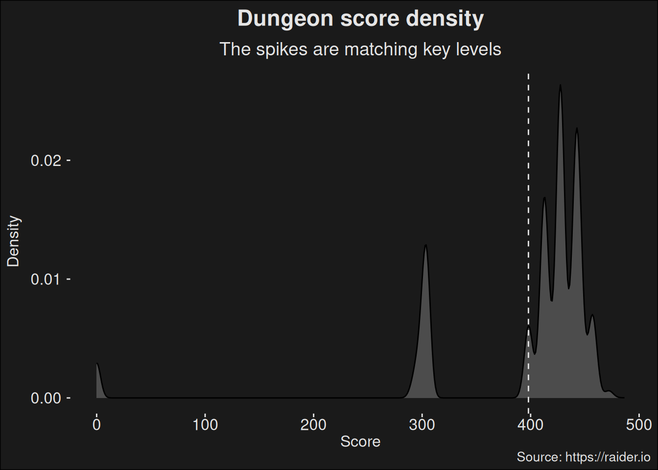
Let us start by looking at a density curve, just to get an early overview of what is going on. While here, compute a mean score and draw it as a dashed line.
Figure 7.1: Overall kernel density of scores for dungeon runs, where all the dungeons are grouped together into one big set of data. This gives a view of where the top players are relatively speaking. The dashed line is the mean. Density plots provides a continuous variant of a histogram, which is often a better way to depict a distribution.
Dungeons have a clear indication of being artificially scored. Each Mythic+ key level has it’s own scoring spike in the plot, and they are separate. This makes the data clearly non-normal in nature.
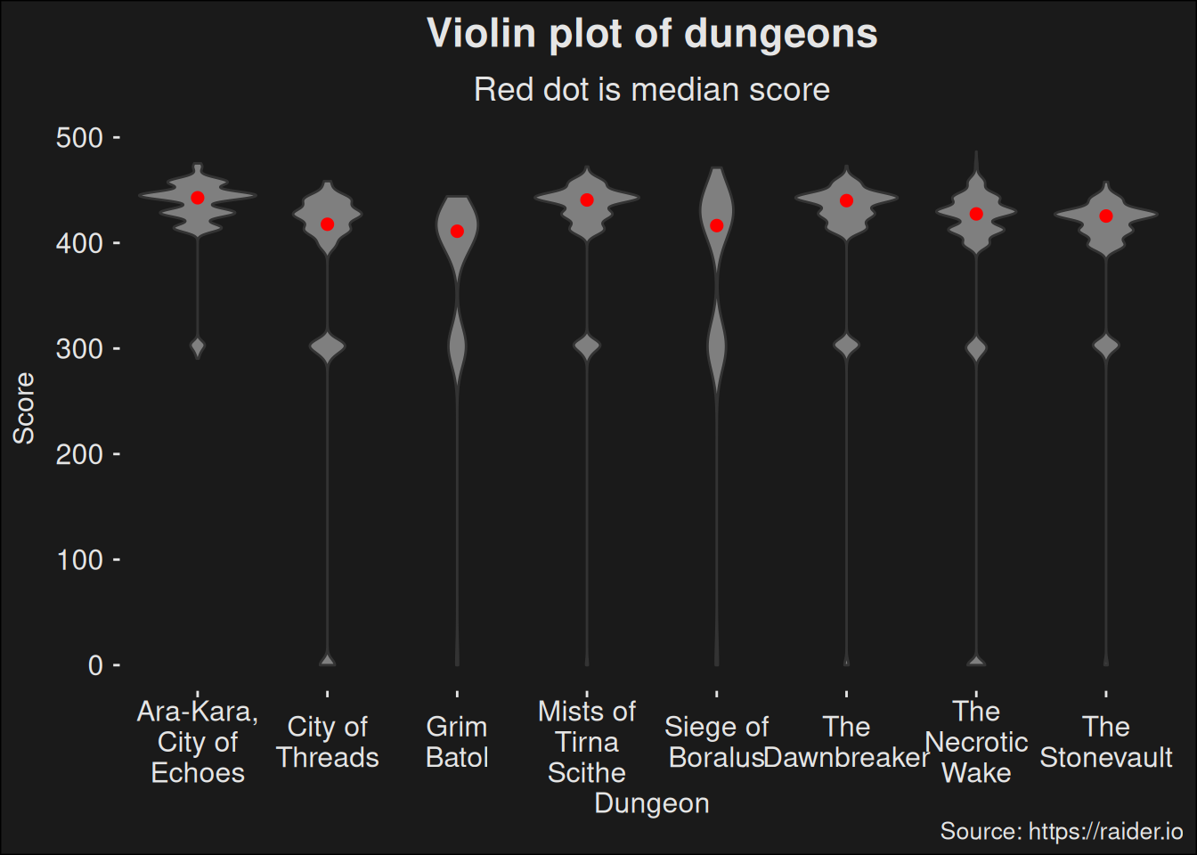
It would be natural to ask questions about data grouped by dungeon.
Code
dungeons |>ggplot(aes(x = dungeon.str, y = score)) +geom_violin(fill="grey50") +stat_summary(fun=median, geom="point", color="red", size=2) +labs(title ="Violin plot of dungeons",subtitle ="Red dot is median score",caption ="Source: https://raider.io",x ="Dungeon",y ="Score") +scale_x_discrete(labels = scales::label_wrap(10))
Figure 7.2: Densities split by dungeon and plotted as a violin-plot. Red dots depict the median of each distribution.
We see a clear indication of dungeon differences. Some dungeons are easier than others and are able to run at a higher key level across the board. This is particularly true when you look at the median scores of the dungeons. They fall over several different typical key levels, so the difference is pretty stark. As a first approxmation the differences in median can be used as a rough tier-list of dungeons.
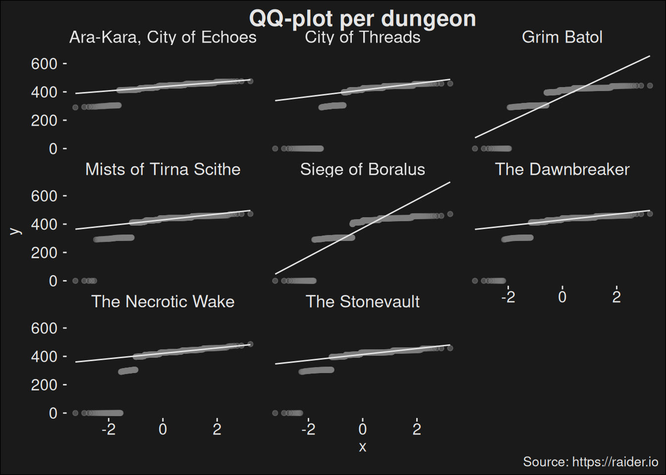
One of the first things to ask is if the dungeon data we are seeing is normally distributed. One way of attacking this question is to look at a QQ-plot1:
1 A QQ-plot is a Quantile-Quantile plot. It plots two distributions against each other. If they agree, the data will fall on a straight line. Usually, one distribution stems from our observed (sampled) data, where the other distribution is some theoretical distribution we want to match against, most often a normal distribution. See Q-Q plot
Figure 7.3: Q-Q plot split per dungeon. The normality varies a bit from season to season and how far we are into a season.
If data is normally distributed, it would fall very close to the line. This data has some very clear influence from the key level, which creates a “stair case” in the plot.
7.2 Regional dungeon differences
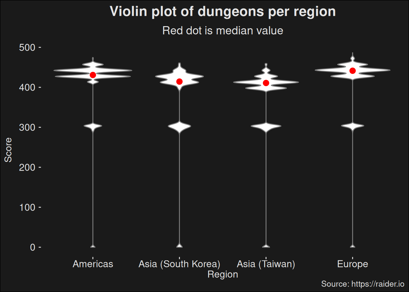
Because we are fetching dungeons from each region, it is worth asking if there is a difference in the regional data:
Code
dungeons |>ggplot(aes(x = region.str, y = score)) +geom_violin(color ="grey50") +stat_summary(fun=median, geom="point", color="red", size=3) +labs(title ="Violin plot of dungeons per region",subtitle ="Red dot is median value",caption ="Source: https://raider.io",x ="Region",y ="Score") +theme(legend.position ="none")
Figure 7.4: Dungeon scores, split by region and plotted as a violin-plot. This plots shows how the scoring varies among the regions, which is important to consider if you want to analyze the top-k runs worldwide.
The plot argues there are considerable regional differences. This is likely because there are fewer players in the Asian regions compared to the Europe and Americas regions. A highly active region is able to push keys to a higher level than one which is less active. In any case, using the top players from each region is wrong insofar we aren’t measuring the top players anymore. The players from Asia provides a push/pull effect on the distribution, due to a differing skill level in that region.
If we want to analyze the top players, we should introduce a different dataset in which we are gathering the worldwide top runs across regions. If most of these runs happen to be in the Europe region, we should just have more runs from Europe in the data.
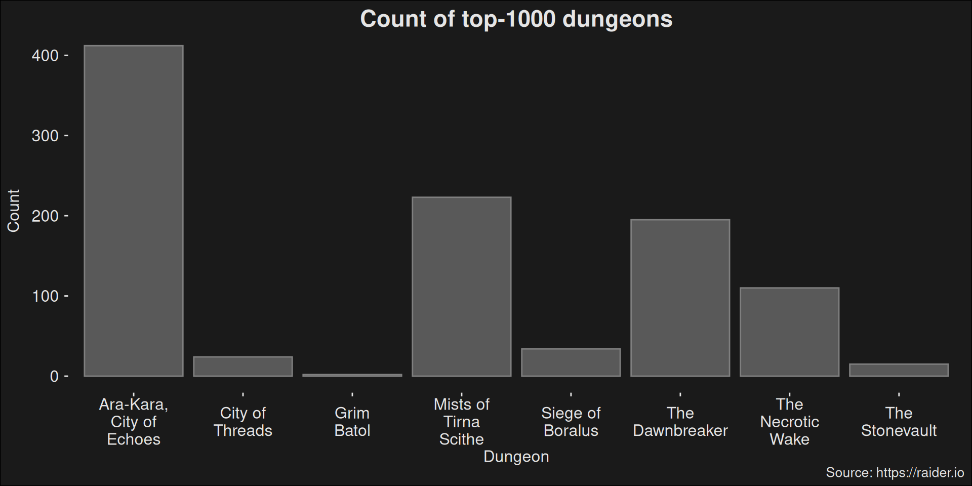
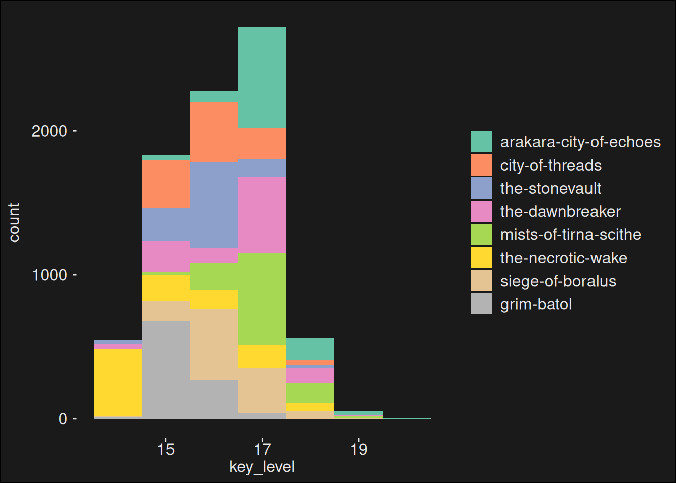
This dataset is prepared by our dungeon-importer. Lets look at the breakdown of the top-1000 dungeon runs in the data set.
Figure 7.5: Find the 1000 dungeon runs with the higest score for the week and count how many there are of each dungeon. The plot is an indicator of overall dungeon balance. If a dungeon occurs rarely in this data set, it is generally considered more difficult than dungeons occurring more often.
Oops! If we look at the runs, it becomes clear we included way more of the easier dungeons. This can vastly skew the estimates on specializations because it ends up measuring more on the easier dungeons. A violin-plot of these dungeons tell a great story about how hard the dungeons are:
Code
dungeons_topk |>slice_max(score, n =1000) |>ggplot(aes(x = dungeon.str, y = score)) +geom_violin(color ="grey70") +labs(title ="Violin plot of dungeons",caption ="Source: https://raider.io",x ="Score",y ="Density") +scale_x_discrete(labels = scales::label_wrap(10))
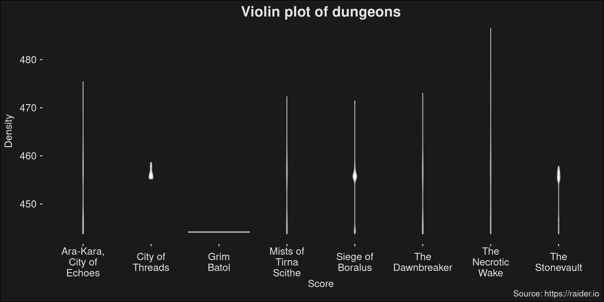
Figure 7.6: Violin-density plot of the top-1000 dungeon runs ordered by score.
For some dungeons, all of the probalitity mass is spread out by a lot, but for other dungeons, the probability mass is compressed into a small region. This makes a choice of focusing on a few top dungeon runs a bit dangerous, if we don’t stratify over all dungeons. We’ll end up with a worse image of what is going on.
7.3 Kobold Analysis
You no take candle!
The first analysis done here is rather weak. It uses some quite basic strategies for analyzing a data set which doesn’t rely on many assumptions about the data. The “real” analysis is to be found in Section 7.5, and you could skip to that section.
The Kobold way of analyzing a dataset like this is rather crude. There’s enough observations, so our data analysis can assume the data is normal. This lets us set up regression analysis among the dungeons.
The way this works is that we set up a null-hypothesis (\(H_0\)) which states there are no difference between the dungeons. We then analyze the dataset to see how likely it would be we got this data by random luck. If this is highly unlikely, we reject the idea of the null hypothesis, which supports the alternative hypothesis that there are differences between the dungeons. To quantify “highly unlikely” we use p-values, where \(p\) is the probability our observations occurs by a random process. The typical cutoff value is \(p < 0.05\) which means that if the observations occur by randomness less than 1/20, we deem there to be a significant effect. We say that the difference is statistically significant.
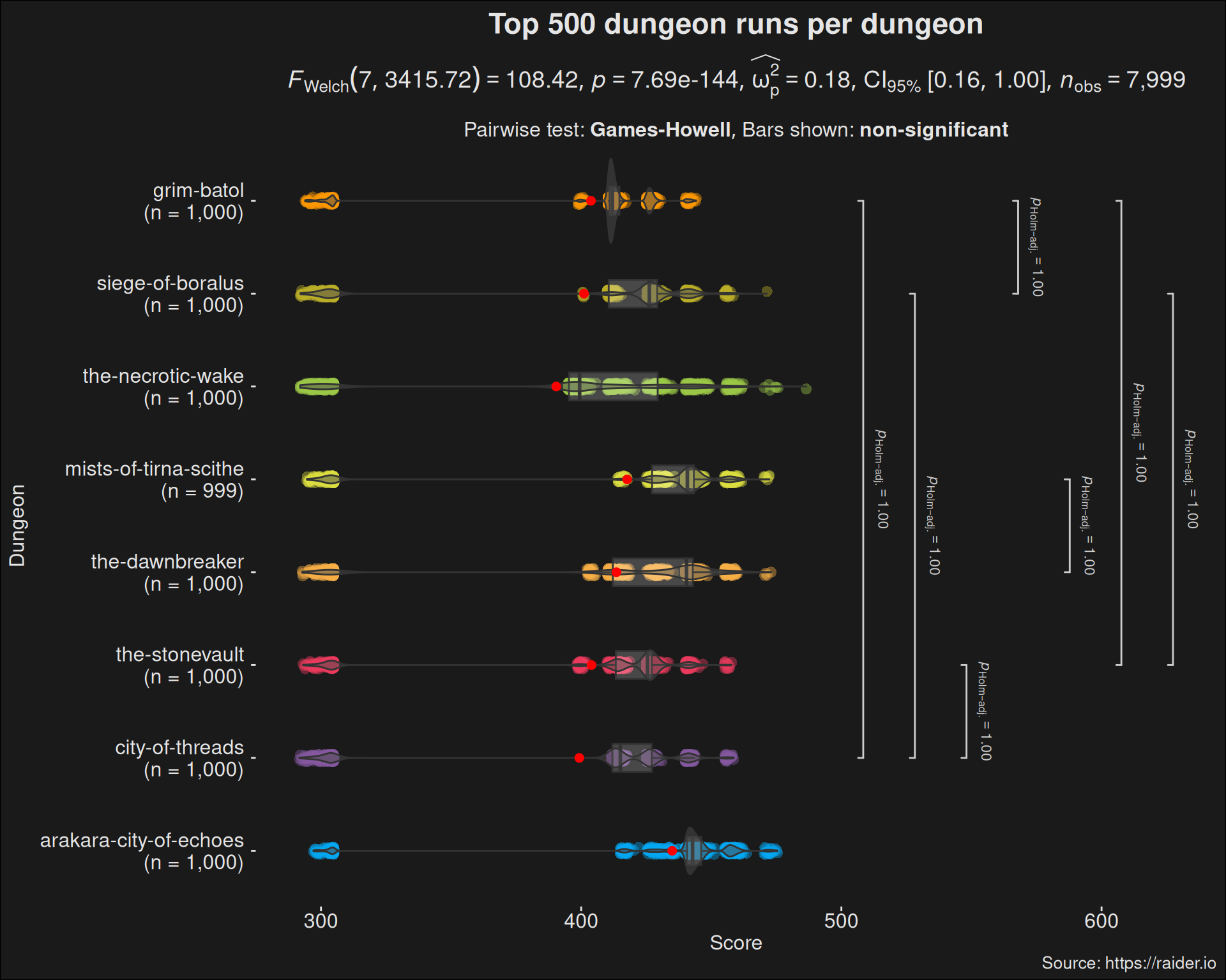
We can summarize the output of the test in a plot directly, by using the ggstatsplot package:
This test only tells us that there are some groups which are different. The test does not tell us which groups. To figure out which dungeons differ from each other, we have to run a so-called post-hoc test. Because there are differences between most of the dungeons, we put a bracket when we fail to show any significant difference. Thus the bracket marks dungoens which are largely equal in difficulty.
The idea of pairwise comparison improves upon Subcreation’s Tier lists. We might have situations where some dungeons are too close in the data and has too much score overlap for us to say that they are different. But it isn’t given you can rank dungeons from best to worst, or give them tiers. It is far better to compare each dungeon to all the other dungeons, by pairing dungeons. However, the number of such comparisons are \(\frac{8 \cdot 7}{2} = 28\) so reporting them all isn’t that feasible.
When we do multiple comparisons, we have to do a p-value adjustment. The problem is the following: suppose there were no difference among the dungeons. Now, if we ran 20 such experiments, then on average 1 of them would show a difference randomly. That’s how we’ve set up our cutoff of \(p < 0.05\). However, if we keep asking different questions on the same data, then about \(1/20\) times, it would reject the \(H_0\) of our question! This phenomenon is called p-hacking, and p-hacking is rather bad. If you keep digging, you’ll randomly strike gold.
The way you get around p-hacking is to require \(p\) to be smaller, the more questions you ask. That way, you can keep controlling for the randomness, even when you ask multiple questions on the same data, as we do with pairwise comparisons. We use an adjustment to parry against p-hacking.
7.4 Goblin Analysis
Warning
This section is currently somewhat weak from a results-perspective, because the checks for the model is failing. This means the results cannot be relied upon, however nice they are looking. In the end, you might want to skip to Section 7.5 where things are on more stable ground.
Goblins are smart, and Goblins use modern statistics. Drawing pentagrams with candles only gets you so far.
The goblin idea is to build a model and then fit the model to the data. Here, the model is a mathematical structure which has well-known properties. The model is an idealized version of our real observations. And the better the fit between data and model, the better the model describes what we saw.
The wise Goblins have deducted that data contains a lot of noise. But inside that noise is a signal—possibly faint—we would like to find. Models work by separating data into different piles (terms). The major idea is that some piles will contain the signal, and other piles will contain the noise. If this separation is clean, we’d be able to read off the signal-terms, while ignoring the noise-terms.
If you happen to find a nice bottle of Kaja’Cola, you might start getting the right ideas. The way Mythic+ dungeons are scored is that the key level determines a base score. This base-score is then adjusted based on how quickly the dungeon is completed. The more time left on the clock, the higher the score2. But care has been taken such that timing a dungeon at the next higher key level scores better than a really quick dungeon run.
2 At lower key levels, untimed keys can still yield some score as long as it is close to the time limit. But at higher key levels, there is no such thing, and untimed keys yields no score. This design prevents a meta-game where one depletes keys for higher score
3 There’s another way to compute this where you use 50% and 150% score, but in the end it’s just a question of where your frame of reference is. The end result is ultimately the same
There is a base score for completing a dungeon, and every key level adds a flat amount of score. The score is further adjusted by how many affixes are in play, and if the party was quicker or slower than the timer allows. Finally, you gain score for both Tyrannical and Fortified weeks, where your best run yields full score, and the other week yields score at 33% value3
This is where the scheming goblin realizes something. Score is heavily predicted by key level and time. It is even a linear relationship. The reason scores clump together in the density plots is because that’s a given key level. This idea is rather obvious. A kobold might dismiss it as being irrelevant. But a goblin realizes the power of this straightforward observation.
Suppose we build a simple linear regression model where score is predicted by key level. We know this is wrong, as the above calculation isn’t linear. It’s also not what we want. We want score predicted by dungeon. But the Goblin assures us this is the way to go.
Code
model_pre_1 <-lm(score ~ key_level, data = dungeons_topk)
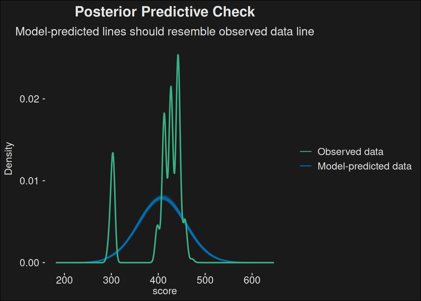
Now, we go in the reverse direction. We use the model to simulate data. We want to see how close the simulated data fits to the observed data.
Code
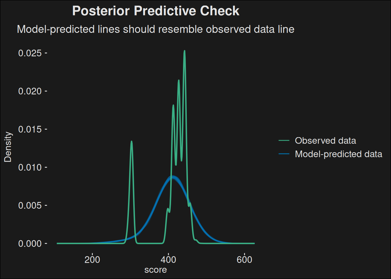
plot(pp_check(model_pre_1))
The goblin is giggling, because they knew. Predicting the score by key level is awfully close to the data we observe. It isn’t what we want, but it captures a lot of the structure of our data. However, the Goblin has a multiple linear regression gizmo. What if we predicted the score based on both the key_level and the time remaining?
Again, we simulate the model against our observed data:
Code
plot(pp_check(model_pre_2))
The fit is even better, but it isn’t perfect. That Goblin is onto something here, smart as they are. Score is derived from the key level and dungeon timing. If we make a model using those inputs, it fits well, even though the scoring computation isn’t entirely linear. This means score is probably the wrong thing to look at, since it is being derived from the key level and how much time was left.
If we want to look at differences between dungeons, we should probably look at either the key level or the time remaining in the dungeon. Time remaining sounds like the wrong predictor, so we are going to use key level instead.
7.4.1 Key level
The key levels plotted per dungeon should give us a good idea of what is going on:
Code
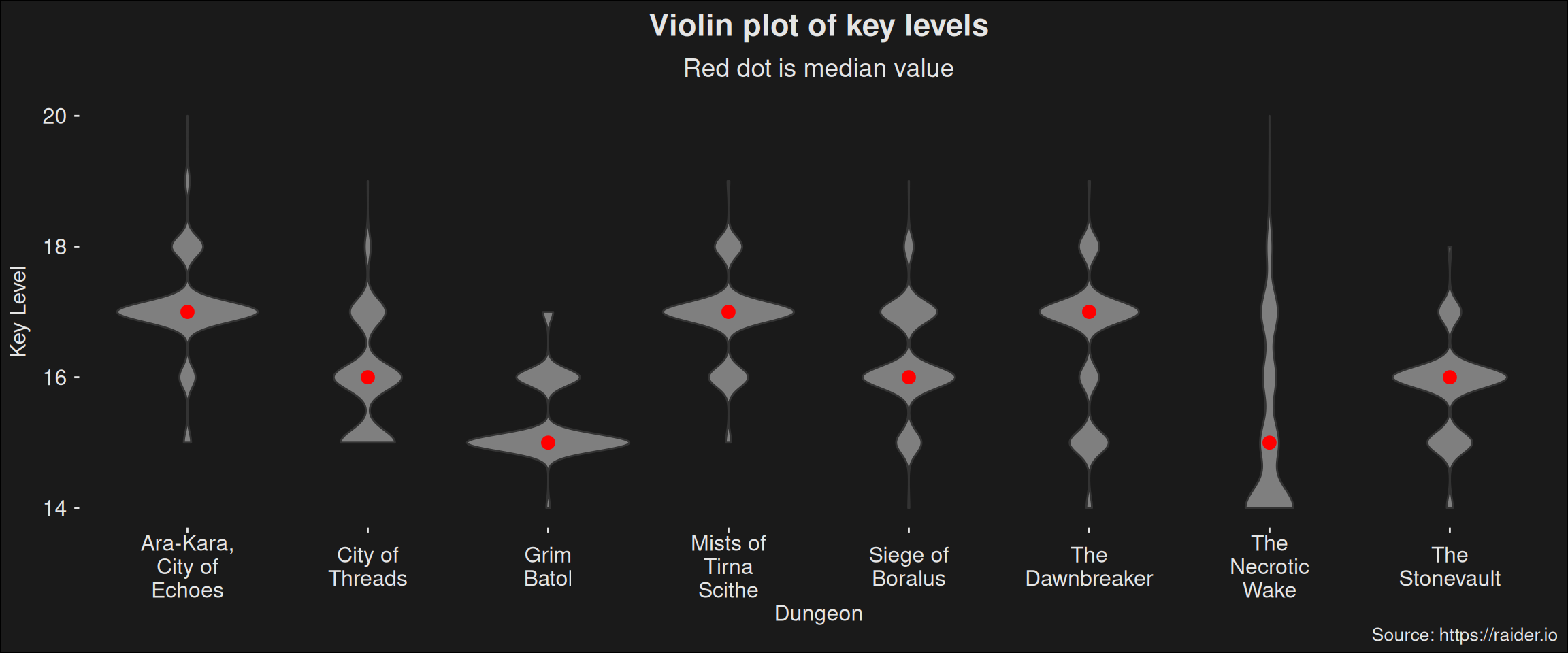
dungeons_topk |>ggplot(aes(x = dungeon.str, y = key_level)) +geom_violin(fill ="grey50") +stat_summary(fun=median, geom="point", color="red", size=3) +labs(title ="Violin plot of key levels",subtitle ="Red dot is median value",caption ="Source: https://raider.io",x ="Dungeon",y ="Key Level" ) +scale_x_discrete(labels = scales::label_wrap(10))
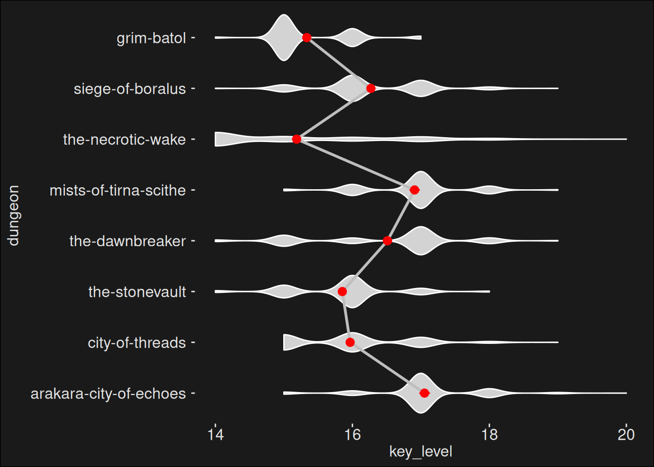
Figure 7.7: Plot of key levels for each dungeon as a violin-plot. This tells us what key levels the dungeons are generally being run at.
Clearly, some dungeons are run at a higher key level than other dungeons. This could give rise to a better model, where we are trying to build a relationship between the dungeon and the key level.
The time remaining in dungeons are likewise interesting. We can plot each runs time remaining as a dot, but jitter them a bit to prevent some overplotting. This allows us to see the numbers are all over the place.
Code
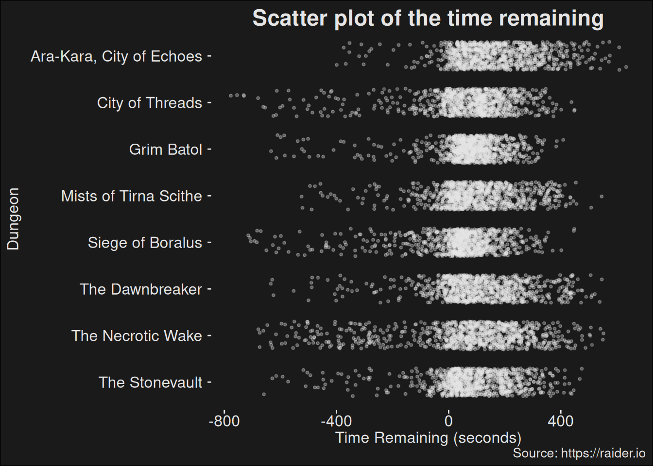
dungeons_topk |>ggplot(aes(x =fct_rev(dungeon.str), y = time_remaining_ms /1000)) +geom_jitter(color ="grey90", size = .75, alpha = .33, width = .3) +coord_flip() +labs(title ="Scatter plot of the time remaining",caption ="Source: https://raider.io",x ="Dungeon",y ="Time Remaining (seconds)")
Figure 7.8: Plot of the time that’s remaining for each dungeon. Each dot corresponds to a run. The X-axis is the time that’s remaining for the run. The Y-axis is the dungeon. Each dot is jittered within a band; placed randomly in the band. This avoids overplotting and makes it easier to see where the mass is. Note: this isn’t the best plot for this data because it doesn’t control for key level. So all key levels are mashed together in this plot.
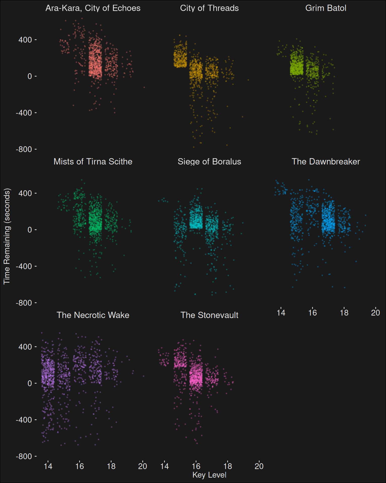
A better plot is to take the key level into consideration:
Figure 7.9: Plot of key level vs time remaining for each of the dungeons. Each dot is a run for the given dungeon. The X axis are key levels. The Y axis is the time reamining for that run. Dots are jittered in a band for each key level. This is done to avoid overplotting.
It looks like as dungeon key levels increase, they get harder to time.
7.4.2 Random effects from groups
More Kaja’Cola. Let us try to predict the key level given dungeon:
This model is a rat. It fails to account for the fact that the same group might run dungeons more than once per week. In fact, some groups run a lot of dungeons. Let’s see how many:
The problem is that groups, tanks, and healers are violating the assumption of independence. For some groups, we will only have a single observation, whereas for others we’ll have more than 20. That is, there are clusters based on the groups in the data set. This means the estimation of the dungeon difficulty might be influenced by a well-playing or badly-playing group which is very active. A ratty solution would be to pool all the runs by a group into a group-mean and then use this to offset the difficulty. It is what we did as a quick solution in the Subcreation chapter. But we can do better. We want groups with few runs to use information from a “global” mean key level score, whereas groups who play more should be less influenced by this global mean. And we want to account for groups playing consistently above/below the grand mean.
It leads to us using a mixed-effects linear model, which supports a partial pooled solution:
Across runs, we believe the dungeon difficulty remains constant. If a dungeon is hard for one group, we believe it is also hard for a different group. That makes a dungeon into a so-called fixed effect.
Across runs, we believe there is a difference between groups. Some groups are better at running dungeons than other groups. And some groups are far more active than other groups. We think the group effect is present on all dungeons they are running: if they are doing good at one dungeon, the same group will also have an easier time with another dungeon. This leads us to model the group as a random effect.
Likewise, we think that healers and tanks might contribute to the key level. The presence of a certain healer or tank in a group might make timing the dungeon easier or harder.
The notion of fixed vs random effect is a bit vague in the literature. There are many different views of what they are, and those views are all attempted explanations of the underlying math. The math has to do with correctly handling the above partial-pooling conundrum. We don’t want to pool everything into one global key level estimate. And we don’t want to do no pooling at all. We want a healthy middle ground, and that’s what a random effect is, roughly.
The idea is that we have a dungeon difficulty which gives us a given key level for the dungeon. But we think a given group can influence this a bit in the positive or negative direction. So if we focus on a given group, the estimated key level might be slightly different. So we posit that the deviation from the global dungeon mean key level follows a (gaussian) distribution.
This model treats groups as having a random effect on the intercept of the linear model. This can be thought of as modeling each group invididually, so a group cannot affect the grand mean score too much. The value \(\tau_{00}\) in the above is the variance from groups. I’d say this is a moderate effect which should be taken into account, given the variance of the full data (\(\sigma^2\)).
Given a model, we can use it to estimate a mean value (marginal mean). Raw data means can be influenced by hidden interactions or spurious data which might occur. The idea of estimated marginal means are they are derived from a statistical model instead. If the model fit is good, then the estimation from the model can avoid some of that noise from the raw mean. Comparing the estimated mean to the raw mean is often a good way to figure out something about the data set.
Code
model_2_means <-estimate_means(model_2)
We selected `by = c("dungeon")`.
Note: D.f. calculations have been disabled because the number of observations exceeds 3000.
To enable adjustments, add the argument 'pbkrtest.limit = 7999' (or larger)
[or, globally, 'set emm_options(pbkrtest.limit = 7999)' or larger];
but be warned that this may result in large computation time and memory use.
Note: D.f. calculations have been disabled because the number of observations exceeds 3000.
To enable adjustments, add the argument 'lmerTest.limit = 7999' (or larger)
[or, globally, 'set emm_options(lmerTest.limit = 7999)' or larger];
but be warned that this may result in large computation time and memory use.
Code
model_2_means |>kbl() |>kable_styling()
dungeon
Mean
SE
CI_low
CI_high
arakara-city-of-echoes
16.59901
0.0238675
16.55223
16.64579
city-of-threads
15.81680
0.0245409
15.76870
15.86489
the-stonevault
15.67659
0.0239450
15.62966
15.72352
the-dawnbreaker
16.27362
0.0240074
16.22656
16.32067
mists-of-tirna-scithe
16.46060
0.0239470
16.41367
16.50754
the-necrotic-wake
15.21108
0.0251669
15.16175
15.26040
siege-of-boralus
16.08224
0.0239670
16.03527
16.12921
grim-batol
15.25791
0.0243992
15.21009
15.30573
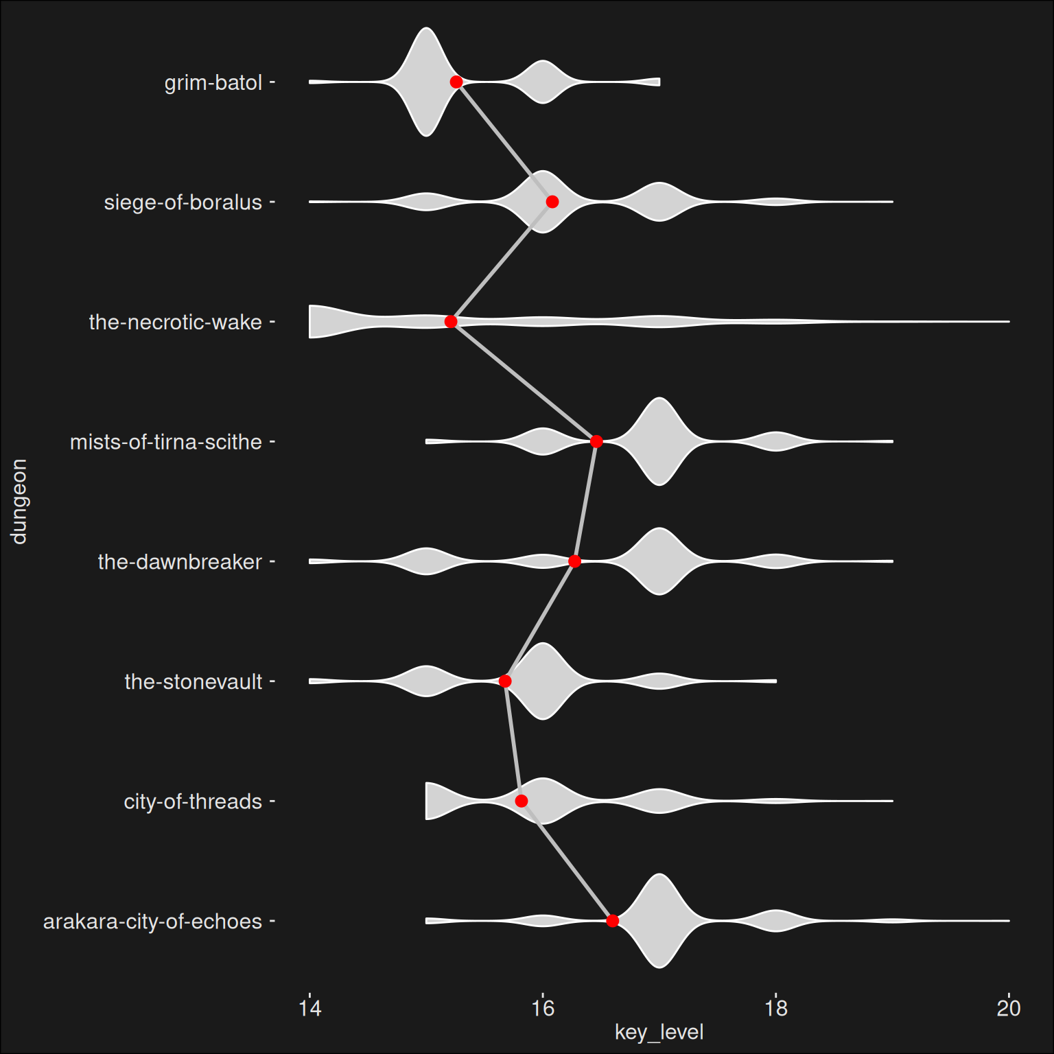
And given these means, we can visualize them on the dungeons directly:
Code
dungeons_topk |>ggplot(aes(x = dungeon, y = key_level)) +geom_violin(fill="lightgray", color ="white") +geom_line(data = model_2_means, aes(y = Mean, group =1),linewidth =1, color ="grey") +geom_pointrange(data = model_2_means,aes(y = Mean, ymin = CI_low, ymax = CI_high),linewidth = .5,color ="red" ) +scale_fill_material_d(palette ="light") +coord_flip()
Note the confidence intervals on the means are quite small. We’ll check if that’s the case later with a different modeling approach.
7.4.3 More random effects
Our dungeon data contains a lot of noise. In a naive model, we’d just suck up all that noise in a grand error-term. But when we model groups separately, we’re able to separate the noise into a group part, and the remaining noise. That is, we try to improve the precision of the model, by taking groups into account.
We can try the same, but use healers, tanks, and dps as 3 separate cluster groupings. That way, we can model the impact of healers, tanks and dps on the key level outcome. This is useful, because if you have a player who are consistently performing better or worse than the average, we can capture that in the model. The cluster is a player, so if the player played more than a single dungeon, we are capturing that in the model rather than treating the players runs as independent.
Clustering dps requires some feature engineering, because there are 3 dps players. We just create a canonical identity for the 3 dps as a group. This isn’t perfect, but it allows for the player to commute and appear in any order in the party.
We can now estimate the means marginally via the model, rather than via the raw data.
Code
m3_means <-estimate_means(model_3, at =c("dungeon"))
Warning: The `at` argument is deprecated and will be removed in the future.
  Please use `by` instead.
Note: D.f. calculations have been disabled because the number of observations exceeds 3000.
To enable adjustments, add the argument 'pbkrtest.limit = 7999' (or larger)
[or, globally, 'set emm_options(pbkrtest.limit = 7999)' or larger];
but be warned that this may result in large computation time and memory use.
Note: D.f. calculations have been disabled because the number of observations exceeds 3000.
To enable adjustments, add the argument 'lmerTest.limit = 7999' (or larger)
[or, globally, 'set emm_options(lmerTest.limit = 7999)' or larger];
but be warned that this may result in large computation time and memory use.
Code
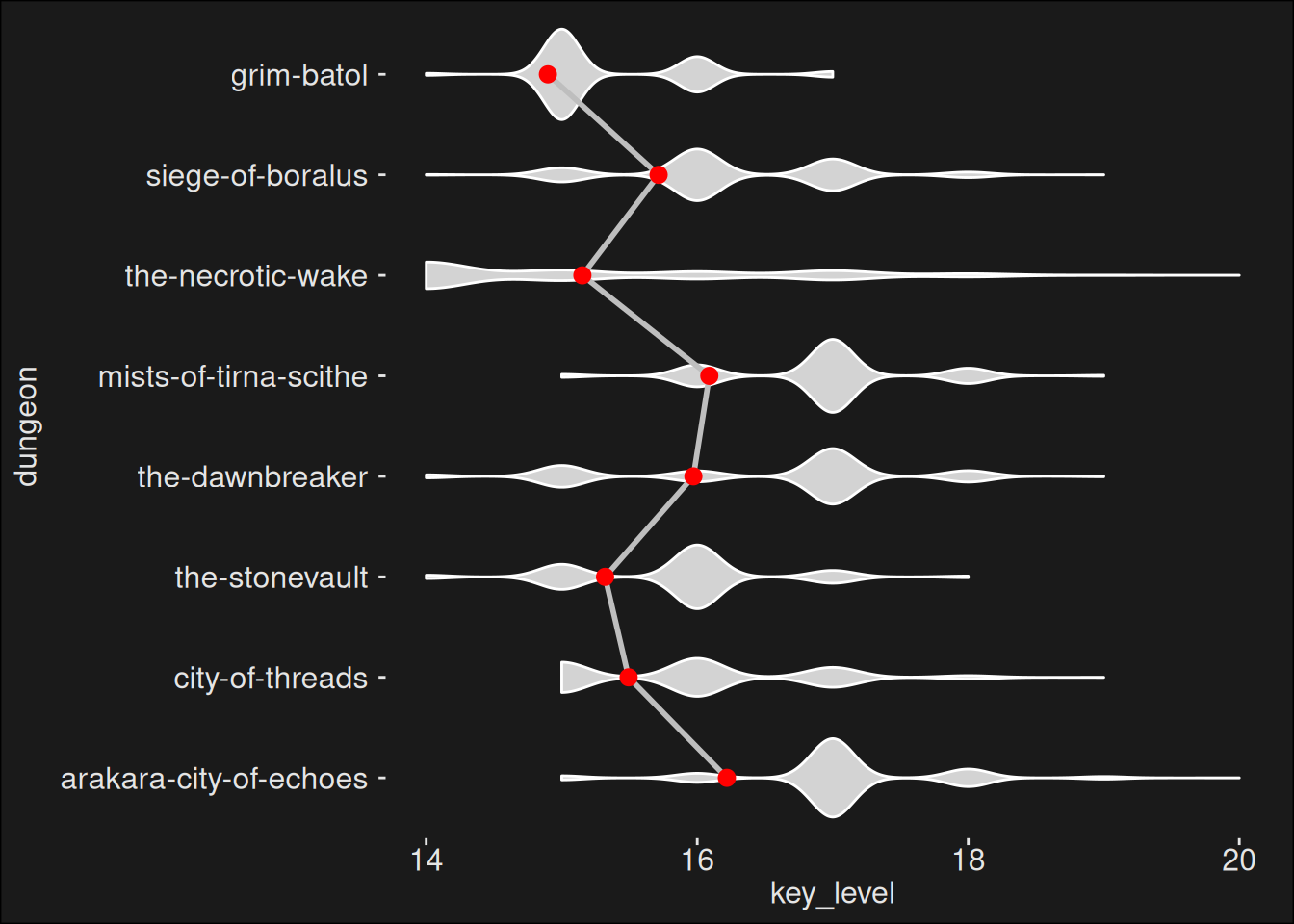
dungeons_topk |>ggplot(aes(x = dungeon, y = key_level)) +geom_violin(color="white", fill ="lightgray") +geom_line(data = m3_means, aes(y = Mean, group =1), linewidth =1, color ="grey") +geom_pointrange(data = m3_means,aes(y = Mean, ymin = CI_low, ymax = CI_high),size = .5,color ="red" ) +scale_fill_material_d(palette ="light") +coord_flip()
We can also use the model to estimate contrasts through contrast analysis. That is, we can look at which dungeon pairings are different and which are the same, statistically. Again, we use a Holm-adjustment to avoid p-hacking the results. Because a lot of these pairings are significant, it is better to report those which are not:
Code
contrasts <-estimate_contrasts(model_3)
No variable was specified for contrast estimation. Selecting `contrast =
  "
  dungeon
  "`.
Note: D.f. calculations have been disabled because the number of observations exceeds 3000.
To enable adjustments, add the argument 'pbkrtest.limit = 7999' (or larger)
[or, globally, 'set emm_options(pbkrtest.limit = 7999)' or larger];
but be warned that this may result in large computation time and memory use.
Note: D.f. calculations have been disabled because the number of observations exceeds 3000.
To enable adjustments, add the argument 'lmerTest.limit = 7999' (or larger)
[or, globally, 'set emm_options(lmerTest.limit = 7999)' or larger];
but be warned that this may result in large computation time and memory use.
We want to improve the model further. To do this, we’ll have to transform the key levels, as we want a different base point. We can center the data so the smallest key is at 1.
   Min. 1st Qu.  Median    Mean 3rd Qu.    Max.
  1.000   2.000   3.000   3.135   4.000   7.000
With the data centered, we can model the response variable as being the centered one. Because the models we’ve used until now are assuming a normal distribution, this rescaling doesn’t have any real effect on those models. However, we can look at generalized linear models, where the distribution isn’t forced to be normal. In particular, we can pick distributions from the so-called exponential family of distributions.
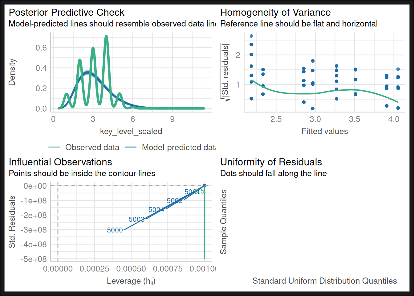
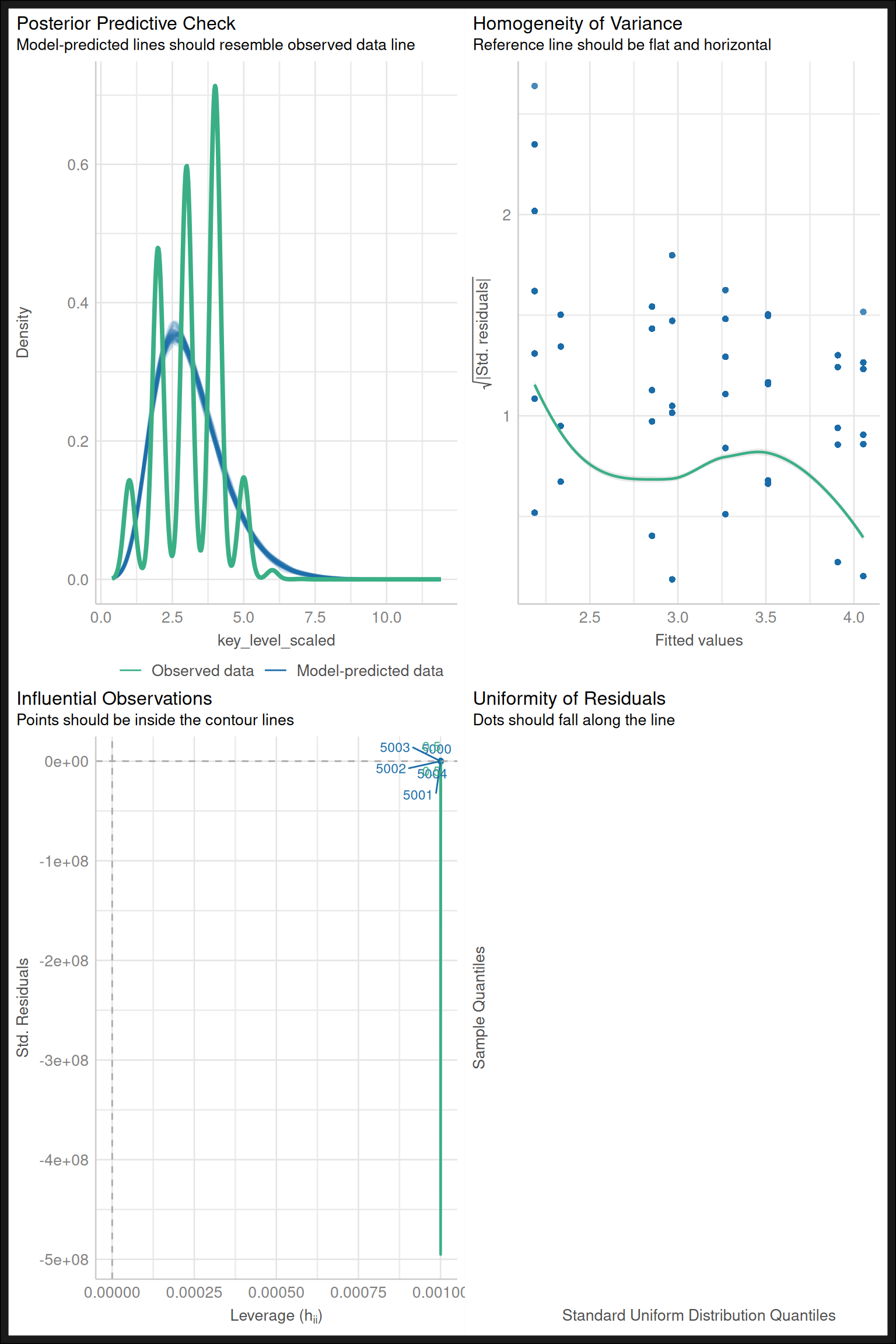
When constructing models, it is important to check them for typical problems. We can create one such a test sheet for our current model:
Code
check_model(model_4)
Typically, we get into trouble with homogeneity of variance, and normality assumptions. It makes the resulting data untrustworthy, and we’d like another view. That view can be provided by the bayesian framework.
7.5 Mechagnome Analysis
Goblin analysis methods are classical methods. Mechagnomes have an alternative way of doing analysis: they throw computers at problems. In our case that means bootstrapping and bayesian methods.
Rather than getting a point-estimate, like a mean, we are going to use the collected data to compute a posterior distribution: the probability of obtaining a certain mean from the data. By throwing compute power at the problem, we’d get some statistics which tend to be more robust against assumption violations as is the example with the goblin approach. This can then be used to make better explanations of the data than what goblins are getting.
The Mechagnome defines their model via bayesian generalized linear regression. The family is a Gamma-distribution, with a log-link:
data {int<lower=1> N; // total number of observationsvector[N] Y; // response variableint<lower=1> K; // number of population-level effectsmatrix[N, K] X; // population-level design matrix// data for group-level effects of ID 1int<lower=1> L; // number of grouping levelsarray[N] int<lower=1> ll; // grouping indicator per observation}parameters {vector[K] b; // population level effectsreal b_m; // population meanreal<lower=0> shape; // shape parameterreal<lower=0> sigma; // variance of the population}transformed parameters {real lprior = 0; // prior contribution to the log posterior lprior += cauchy_lpdf(sigma | 0, 5); lprior += normal_lpdf(b | b_m, sigma); lprior += gamma_lpdf(shape | 0.01, 0.01);}model {vector[N] mu = rep_vector(0.0, N); mu += X * b; mu = exp(mu);target += lprior;target += gamma_lpdf(Y | shape, shape ./ mu);}generated quantities {array[N] real y_rep; y_rep = gamma_rng(shape, shape ./ exp(X * b));}
fit <- cmdstanr::as_cmdstan_fit(res$output_files())
The Mechagnome is thinking that this is a good way to model dungeon runs. You start with all the top groups in the game. Then, whenever you increase the key level of the dungeon by one, there’s some of those groups who will “tap out”, and not be able to play that higher key level. The assumption is that the proportion of groups who stops playing is roughly fixed for every key level increase. That way, we are counting how many key levels the groups manage to get through before they leave for the week.
Or put in another way: we put all the groups into a box. The key levels are time. When we increase time, a certain number of groups “decays”, and we are left with fewer. This happens at a given probability for each group in the box. Thus, the groups form a Poisson Process, much like radioactive particles would.
This leads one to try distributions which can model such particle decays correctly. The Poisson distribution is what particle decay follows, so the Mechagnome thinks this is a good way of modeling dungeon runs.
Furthermore, we use partial pooling over the dungeons. We let the grand overall coefficient for all dungeons have an effect on each of the dungeons.
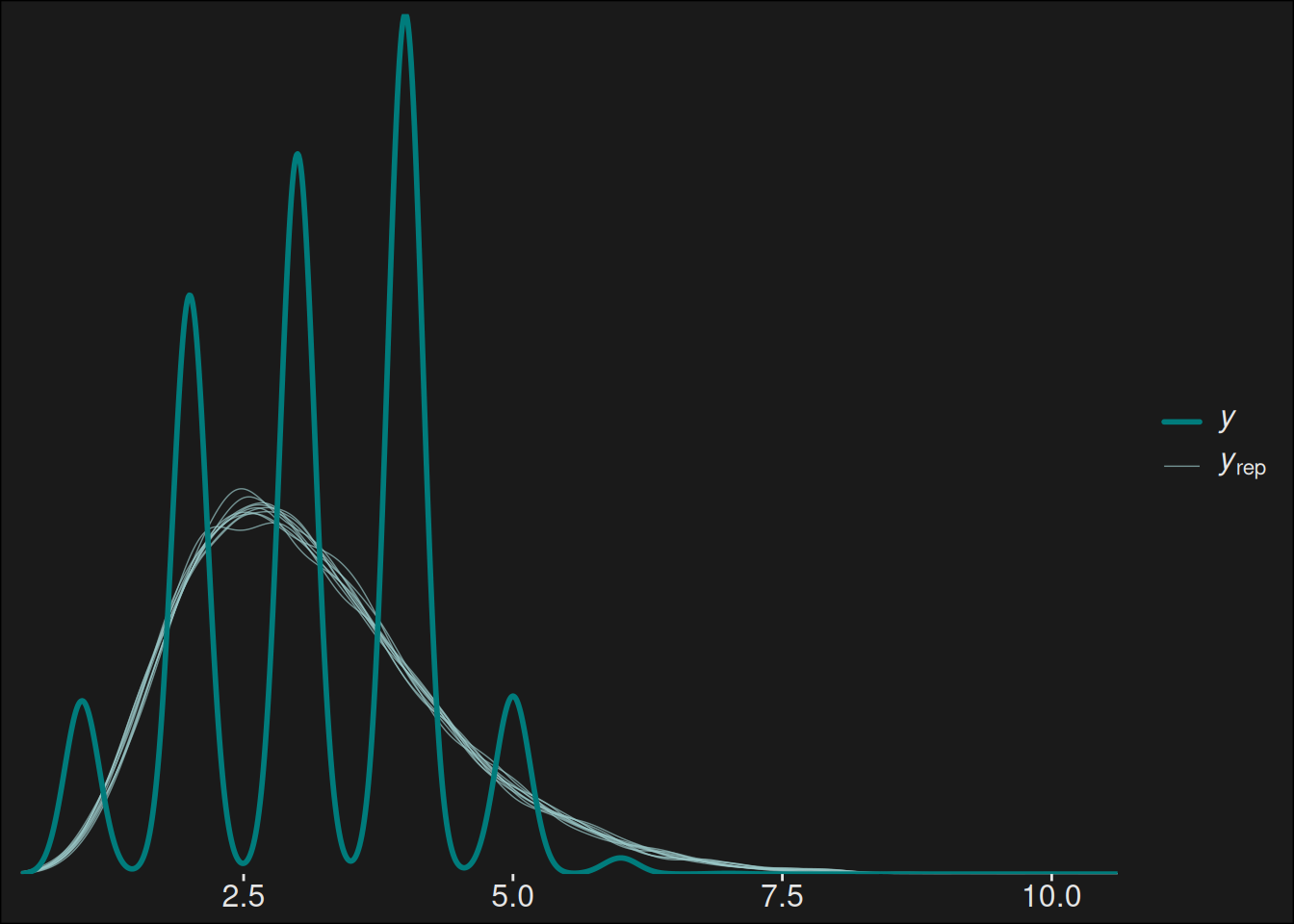
Let us run a posterior predictive check on the data we got:
Code
y <- dungeons_topk$key_level_scaledyrep <- fit$draws("y_rep", format ="matrix")color_scheme_set("teal")ppc_dens_overlay(y, yrep[1:10, ])
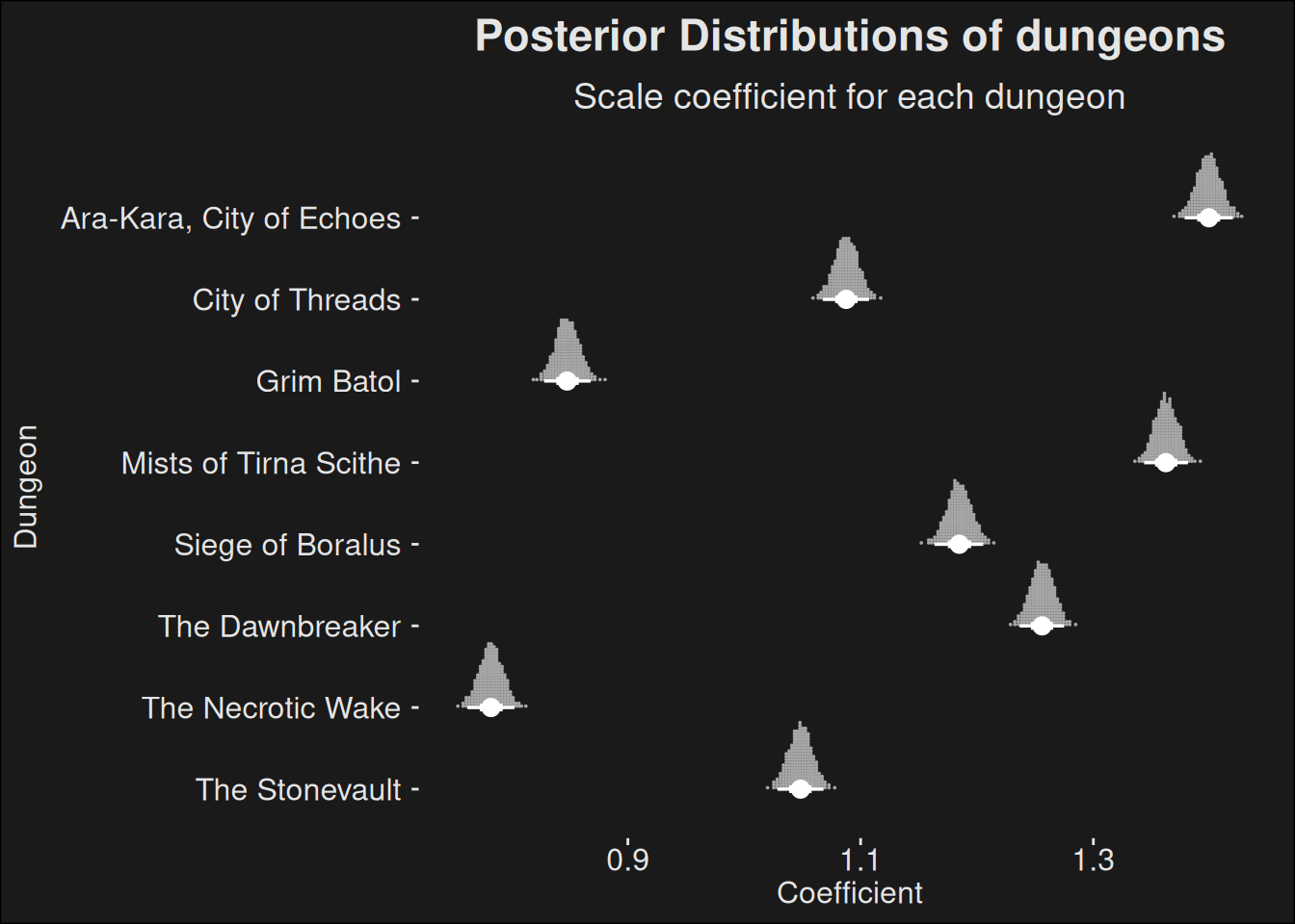
The fit isn’t perfect at all, but it does capture the proportionality somewhat. We can take a look at the data for the dungeons, by plotting the coefficient distributions from the model:
Code
fit |>recover_types(dungeon_data_input |>mutate(dungeon =fct_drop(dungeon))) |>spread_draws(b[dungeon]) |>inner_join(dungeon_names, by =c("dungeon"="key")) |>ggplot(aes(y =fct_rev(dungeon.str), x = b)) +stat_dotsinterval(quantiles =250, color ="white") +labs(title ="Posterior Distributions of dungeons",subtitle ="Scale coefficient for each dungeon",x ="Coefficient",y ="Dungeon" )