This chapter analyzes specializations in a different way. Rather than looking at overall specialization Mythic+ scores, we use data from individual dungeon runs. This is the same approach taken by Subcreation.
The advantage of the dungeon data is that it includes more information about who played in the dungeon. This allows us to build a more complex model which encompasses this extra data. In particular, it allows us to model differences in dungeon difficulty, and differences in player skill.
9.1 Study Design
We first analyze the data and how they nest in each other:
Region
Dungeon (Key Level, Score)
Run
Roster (Bloodlust, Combat Resurrection)
Tank (Class, Specialization, Player)
Healer (Class, Specialization, Player)
DPS 1 (Class, Specialization, Player)
DPS 2 (Class, Specialization, Player)
DPS 3 (Class, Specialization, Player)
Importantly, the Player might repeat1. This happens if a given player plays more of the same dungeon each week.
1 If we don’t do anything about this, players will pseudoreplicate, appearing as if they were independent players. A single player running 7 dungeons that week will look as 7 different players to a naive model. This will vastly skew the results to the point of making them unusable, because when observations are independent, they provide a lot of strength.
9.2 Data Import and preparation
We’ll work with our Top-k-dungeons data for this work.
Code
source('load-specs.R')specs <- specs |>right_join(spec_names, by =c('class_spec'='key')) |>inner_join(region_names, by =c('region'='key')) |>mutate(class_spec =factor(class_spec))specs_topk <- specs_topk |>right_join(spec_names, by =c('class_spec'='key')) |>inner_join(region_names, by =c('region'='key')) |>mutate(class_spec =factor(class_spec))specs_small <- specs_small |>right_join(spec_names, by =c('class_spec'='key')) |>inner_join(region_names, by =c('region'='key')) |>mutate(class_spec =factor(class_spec))
Like in the other expositions, we are going to recenter the data so it starts at 0. This avoids us having to transform data in our stan programs, and makes a Gamma distribution more likely to match. Data pre-processing is fairly common in statistics and machine learning. You want to engineer the data a bit such that it is easier for the model to pick up what is going on.
The whole section here explains the background for the model used, and the considerations of its construction. You can skip ahead to Section 9.4 if you are in a hurry or text doesn’t spark joy.
The data consists of dungeon runs, so in a sense it’s a dungeon data set. We’ve already analyzed dungeons, and we know they have a varying difficulty. Hence, depending on the dungeon you are running, the expected score might vary. Suppose for instance you take a Protection Paladin and a Blood Death Knight with the same Mythic+ score from a dungeon run. You would assume they are about the same. But if you were then told one specialization was running the easiest dungeon in the season, while the other were running the hardest one, you wouldn’t expect them to be the same, even if they have the same M+ score. You would expect the player/spec running the harder dungeon is stronger.
The first idea is thus to model dungeon difficulty.
The second idea is to model player skill/contribution individually. The number of runs by a player varies. You have players with a single run for a week, and players who play more than 20 dungeon runs. Capturing this run variance is important, because those observations are dependent on each other. By clustering all observations from the same player, we can compute a certainty of their skill. We are less certain if the player did few runs, or if the runs aren’t consistently high or low in scores.
It so happens to be each player plays a specialization. Thus players are nested within specializations. We can thus form a hierarchy, where a specialization is the group of players who plays that specialization2. This allows us to estimate a specialization contribution by pooling the player group. This pooling is partial. You have information about a player and “grand” information about all players within a spec. If the player has relatively few runs, we don’t know a whole lot about the player, so we “steal” information from the “grand” spec contribution to make a good guess about our player estimate. Likewise, a player who plays a lot of runs could have enough data to stand on their own. So we’ll take less information from the “grand” spec. That is, partial pooling balances the two extremes where we pool everything into the specialization, or where we do not pool at all, letting each player stand on their own.
2 Nesting players within specializations acknowledges there’s a relationship which cannot be broken. The perceived power of a specialization is dependent on the players who play them. Once the community learns how to play a specialization well, it’ll become more powerful as they min-max the playstyle. Hence, the strength of a specialization is intimately tied to the players who play it. The model used here reflects that by modeling a hierarchy.
The reason partial pooling is so desirable is that it trades off bias and variance. If we pool fully toward a spec, then it introduces a bias toward the (estimated) population mean of the spec. But it also lowers the variance. The lack of pooling avoids the bias, but introduces variance. Partial pooling allows us to tune the tradeoff, based on the data we have. This often leads to a better model fit.
Finally, the data are Gamma-distributed, as we’ve discovered. So we are going to model the response score \(y\) as being Gamma-distributed with some shape parameter. The above considerations controls a scale/rate parameter of the Gamma distribution. The parametrization we opt to use is to model the mean \(\mu\), rather than the usual shape/scale, or \(\alpha\)/\(\beta\) characterizations of the Gamma distribution.
We are also going to log-link our linear model. That is, we are going to work in a log-space and linearize inside it. A log-space has better properties for the data, so it is easier to work in and linearizes the data better. However, the flip side is that some of our results are harder to interpret.
We can write these ideas into a stan program.
9.3.1 Specialization pooling
We have to decide if we should pool the specializations themselves and learn a common variance for them, or if we should let their variance be per-spec. For now, we’ve chosen to pool the variance, but later model exploration and selection could switch this, if a non-pooled model has a better fit to the data.
Both options are theoretically valid. On one hand, you probably don’t want shrinkage where the weaker specs are being pulled in by the stronger specs. On the other hand, there’s less data in some specs, and making an educated guess on the underlying variance, had there been more players playing, could be the right move.
9.3.2 Writing a stan model
data {int<lower=1> N; // total number of observationsint<lower=1> N_player; // total number of playersint<lower=1> N_spec; // total number of class_specsint<lower=1> K; // population level effectsvector<lower=0.001>[N] y; // response variablematrix[N, K] X; // design matrixarray[N] int<lower=0, upper=N_player> player; // Observation -> Playerarray[N_player] int<lower=0, upper=N_spec> spec; // Player -> Spec}parameters {// Overall shape of the Gamma distributionreal<lower=0> shape; // shape parameter// Beta parameters are the effects that happenvector[K] beta; // parameters for X// Players are nested within specsvector[N_player] alpha_player_raw; // Player effectvector[N_spec] alpha_spec_raw; // Specialization effectreal<lower=0> sigma_spec;real<lower=0> sigma_player;}transformed parameters {vector[N_spec] alpha_spec = alpha_spec_raw * sigma_spec;vector[N_player] alpha_player = alpha_player_raw * sigma_player;vector[N_player] alpha_spec_player = alpha_spec[spec] + alpha_player;}model {vector[N] mu = alpha_spec_player[player] + X * beta; mu = exp(mu);// Hyper-priorstarget += cauchy_lpdf(sigma_spec | 0, 1);target += cauchy_lpdf(sigma_player | 0, 1);// Priors// Shape of the gamma distribution curvetarget += gamma_lpdf(shape | 0.01, 0.01);target += cauchy_lpdf(beta | 0, 2);// All these are reparameterized via transformed parameters// to speed up the computation and make it more stable.target += std_normal_lpdf(alpha_player_raw);target += std_normal_lpdf(alpha_spec_raw);// Population model + likelihoodtarget += gamma_lpdf(y | shape, shape ./ mu);}generated quantities {/* array[N] real y_rep; y_rep = gamma_rng( shape, shape ./ exp(alpha_spec_player[player] + X * beta));*/ }
Preparing the data for this program is rather straightforward.
In the stan program, we’ve opted to base the dungeon pillar on a standard (linear) design matrix \(X\), whereas the players/specializations are modeled as a change in intercept. In a design matrix \(X\) one of the dungeons are chosen to be the baseline dungeon, and the other dungeons are modeled as a change from this baseline. This means the first column of the matrix \(X\) is the intercept. The outputs will be a slight nuisance to interpret because of this modeling, but we aren’t interested in the dungeons, so it’s okay.
Another way of saying this is that we are picking a dungeon as a “control group” and for Dragonflight Season 1, we chose “Algeth’ar Academy” because it’s the first one alphabetically. So we assume that dungeon is the baseline, and the other dungeons are varied compared to it’s value.
The reason you don’t put all 8 dungeons in the model and make a separate intercept is that you then have 9 elements describing an 8-dimensional space. Picking 8 of those fully spans the space. Thus the final element would be a combination of the other 8. This leads to trouble in the math, because there’s no way we can get a nice separation anymore. The intercept would end up fighting with one of the dungeons, pushing against each other. This is avoided by taking one of the dungeons as the intercept3.
fit <- cmdstanr::as_cmdstan_fit(res$output_files())
It takes stan some time to complete the \(4000\) samples. But once it’s done, we can look at the data.
Code
ppc_dens <-function(res, dat) { y <- dat$y yrep <- res$draws("y_rep", format ="matrix")color_scheme_set("teal")ppc_dens_overlay(y, yrep[1:10, ])}ppc_dens(fit, spec_data)
9.4 Analysis
9.4.1 Summary
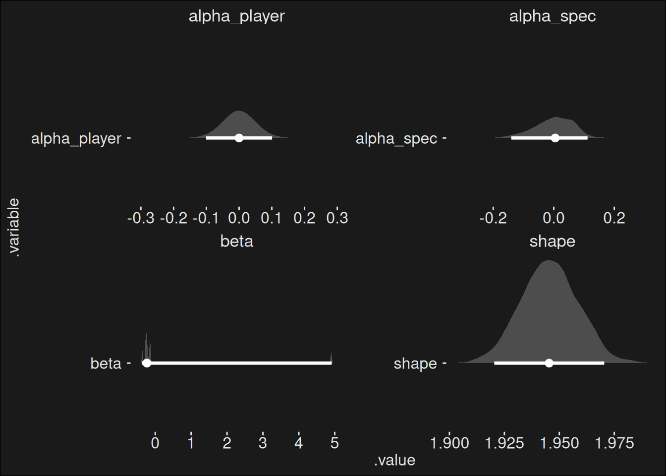
The first plot looks at the parameters, where we gather all dungeons, all player contributions, and all specialization contributions.
Code
summary_analysis <-function(fit) { fit |>gather_draws(shape, alpha_spec[spec], beta[dungeon], alpha_player[id]) |>ggplot(aes(x = .value, y = .variable)) +stat_halfeye(.width = .95, color ="white", fill ="gray30") +facet_wrap(~ .variable, nrow =2, scales ="free")}summary_analysis(fit)
In the plot, shape is the overall shape of the Gamma distribution. The (8) beta-coefficients models dungeon difficulty. Player skills are modeled by the coefficients alpha_player (there’s one for each of the approximately 4000 players). Finally, 38 alpha_spec coefficients models the contribution from each spec.
First, note how dungeons are all over the place. This means the model values the dungeon highly in the computation of a score. This makes sense, as dungeons tend to be quite far apart in difficulty, with some dungoens being far easier than others. In Dragonflight Season 1, the discrepancy was almost two key levels. Not controlling for this in your model is going to mess up the statistics.
Second, note the variance of player contribution is about 4-5 times larger than the spec contribution. This likely means skill matter a whole lot more than spec. There’s a motto in World of Warcraft:
Bring the player, not the class
This motto is likely correct. The player has such a large impact that even if they play the worst spec, they’ll still outperform a more median player on the best spec. And remember this data looks at top dungeon runs. We are looking at something like the 99th percentile of all players, and yet, skill matter far more than the specialization.
The summary analysis describes what the model is doing. We assume the data has a signal (specialization power) and a lot of noise. Then we first model dungeons, which we regard as noise. But because we capture the noise, we can subtract it, and we obtain a better signal/noise ratio in the residual information. Then we model player skill, which we regard as noise. But it largely allows us to subtract player skill as well. That leaves us with even less residual information, in which we hope the signal is strong enough to say something about specialization power.
9.4.2 Player skill
Code
spec_analysis <-function(fit, dat) { fit |>recover_types(dat) |>spread_draws(alpha_spec[class_spec]) |>inner_join(spec_names, by =c("class_spec"="key")) |>ggplot(aes(y =fct_reorder(class_spec.str, alpha_spec),x = alpha_spec,color = key.class)) +stat_halfeye(fill ="gray30") +geom_vline(xintercept =0, color ="white", linetype ="dotted") +scale_color_manual(values = wow_colors) +labs(title ="Posterior Distributions of specializations",subtitle ="Scale coefficient for each specialization",x ="Coefficient, [66%, 95%] CI",y ="Specialization" ) +theme(legend.position ="none" )}spec_rope <-function(fit, dat) { fit |>recover_types(dat) |>spread_draws(alpha_spec[class_spec]) |>inner_join(spec_names, by =c("class_spec"="key")) |>ggplot(aes(y =fct_reorder(class_spec.str, alpha_spec),x = alpha_spec,fill =after_stat(abs(x) <0.05) )) +stat_slab() +geom_vline(xintercept =c(-0.05, 0.05), linetype ="dashed", color ="grey70") +scale_fill_manual(values =c("grey30", "skyblue")) +labs(title ="ROPE for specializations",subtitle ="Which specs lie inside/outside of the ROPE",x ="Coefficient, [66%, 95%] CI",y ="Specialization" ) +theme(legend.position ="none" )}role_analysis <-function(fit, dat, rl) { fit |>recover_types(dat) |>spread_draws(alpha_spec[class_spec]) |>inner_join(spec_names, by =c("class_spec"="key")) |>filter(role == rl) |>ggplot(aes(y =fct_reorder(class_spec.str, alpha_spec),x = alpha_spec,color = key.class)) +stat_halfeye(fill ="gray30") +geom_vline(xintercept =0, color ="white", linetype ="dotted") +scale_color_manual(values = wow_colors) +labs(title ="Posterior Distributions of specializations",subtitle ="Scale coefficient for each specialization",x ="Coefficient, [66%, 95%] CI",y ="Specialization" ) +theme(legend.position ="none" )}role_rope_analysis <-function(fit, dat, rl) { fit |>recover_types(dat) |>spread_draws(alpha_spec[class_spec]) |>inner_join(spec_names, by =c("class_spec"="key")) |>filter(role == rl) |>ggplot(aes(y =fct_reorder(class_spec.str, alpha_spec),x = alpha_spec,fill =after_stat(abs(x) <0.05) )) +stat_slab() +geom_vline(xintercept =c(-0.05, 0.05), linetype ="dashed", color ="grey70") +scale_fill_manual(values =c("grey30", "skyblue")) +labs(title ="ROPE for specializations",subtitle ="Which specs lie inside/outside of the ROPE",x ="Coefficient, [66%, 95%] CI",y ="Specialization" ) +theme(legend.position ="none" )}player_analysis <-function(fit, dat) { core <- fit |>recover_types(dat) |>spread_draws(alpha_player[id]) |>median_qi()union( core |>slice_max(n =30, alpha_player), core |>slice_min(n =5, alpha_player) ) |>inner_join(dat, by =c("id"="id")) |>ggplot(aes(y =fct_reorder(sprintf("%s [%s]", name, spec), alpha_player),x = alpha_player, xmin = .lower, xmax = .upper,color = class)) +geom_pointrange() +scale_color_manual(values = wow_colors) +labs(title ="Posterior Distributions of players",subtitle ="Top-30 and Bottom-5 players",x ="Coefficient [95% CI]",y ="Player" ) +theme(legend.position ="none" )}
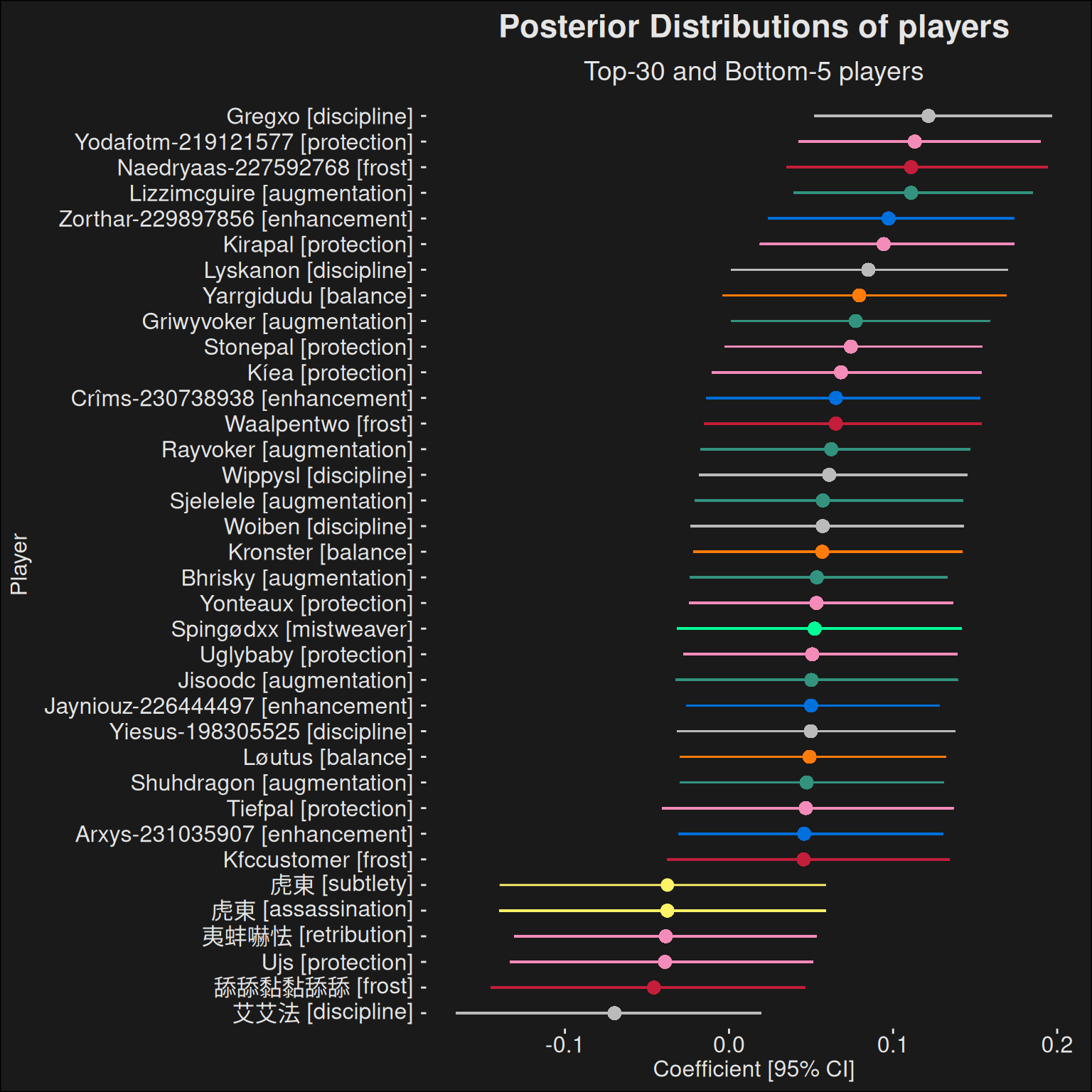
We can take a look at the models player skill computations. There’s about 4000 players in the data set, so we only plot the very top and very bottom players.
Code
player_analysis(fit, data)
Figure 9.1: Player strength as computed by the model. The top-30 players are plotted with the 5-bottom players for reference. For each player, there’s an estimated power and also an estimation of the certainty of that power. A player who plays more, and more consistenly will have a smaller interval compared to a player playing less and with more inconsistency in results.
We’ve plotted the top-30 players together with the bottom-5 players. This shows us how far apart the player contribution is, and what kind of variance to expect for different types of players. The interval is the 95% CI. Note that bottom-5 refers to players who got a top-k dungeon run that week. In the grand scheme of things, they are among the 0.1% of all players playing, and are really really good players. Yet, the plot shows there’s a wide variety in player skill, even among the top players in the game.
9.4.3 Specializations
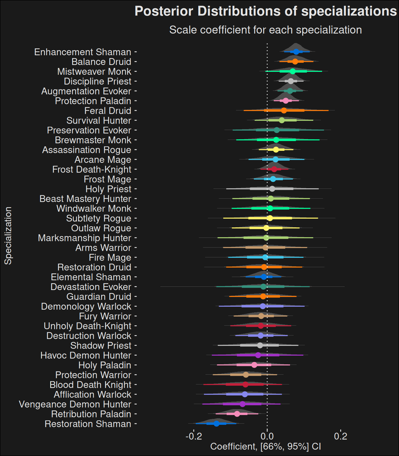
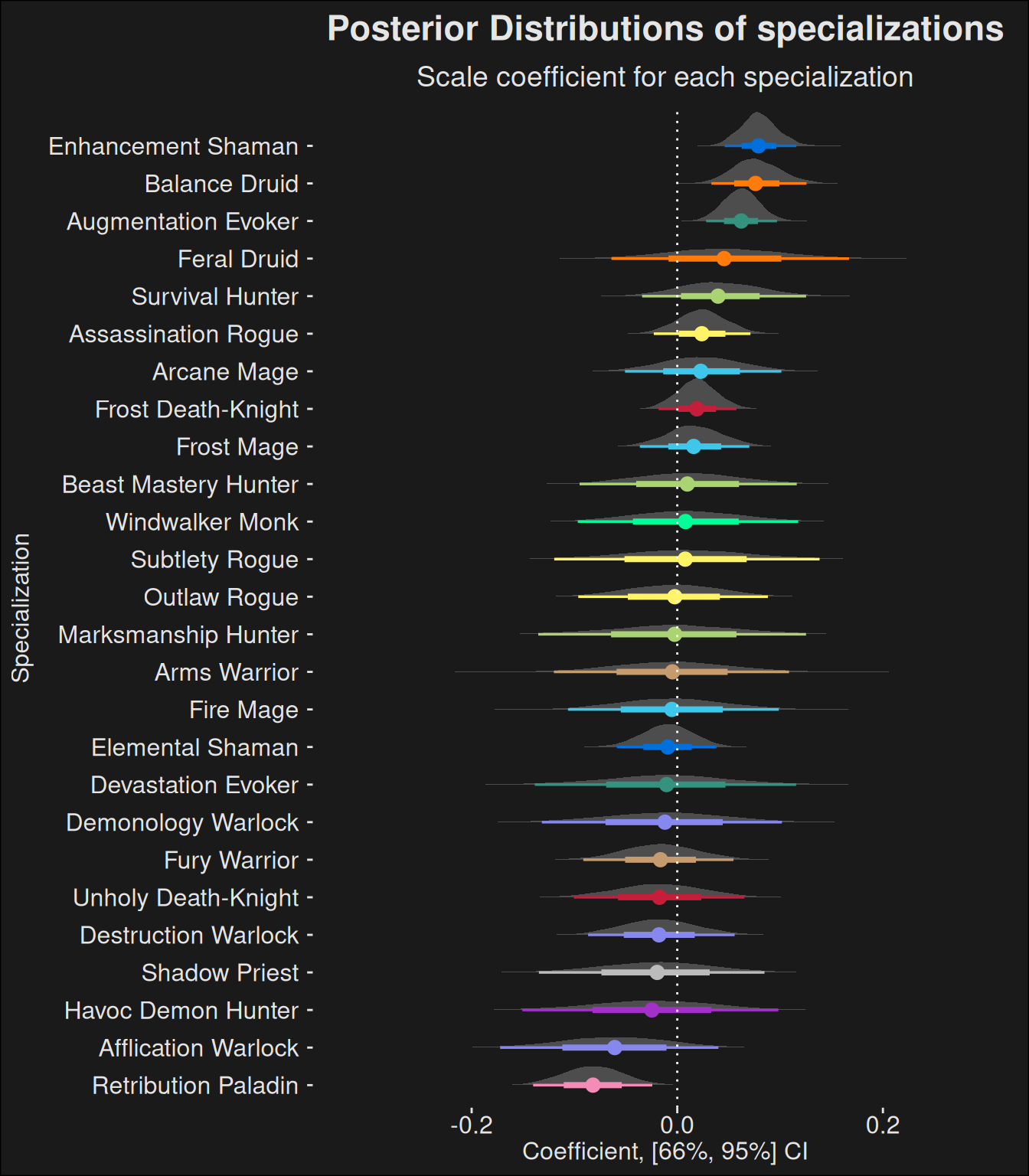
Having controlled for player skill and dungeon difficulty, we can take a look at the data in which players are most interested: the contribution of specializations.
Code
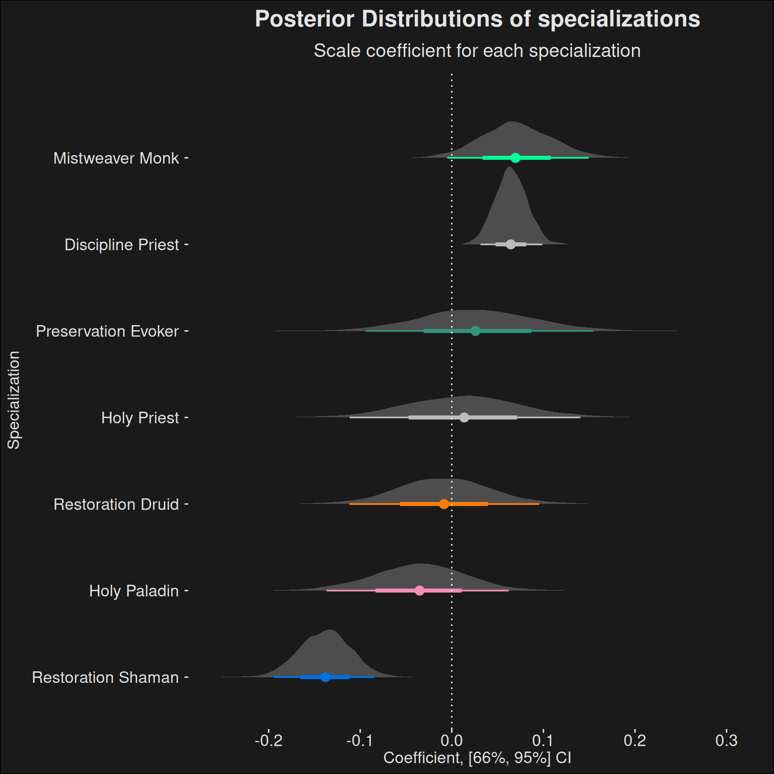
spec_analysis(fit, data)
Note the rather small contribution by each specialization. This is because we are removing the “noise” introduced by dungeon difficulty and individual player skill. Specs which aren’t played that much will have a wider CI, and specs which are highly inconsistent in their contribution will likewise have a wider CI. If the 95% CI straddles zero, then it’s likely the contribution is practically 0, especially since the effect is rather small. It tends to do so for most specializations.
A wide CI-band means we have little information about the spec. This means you should take the power with a grain of salt. If more players would play the spec, we would have a better understanding of its power. Specializations which are above 0 with a wide band are good candidates for being “sleepers” insofar they are strong, but few players are playing them at the top.
If a spec is not stradding 0 with its band, it’s a candidate for being an over/under-performer.
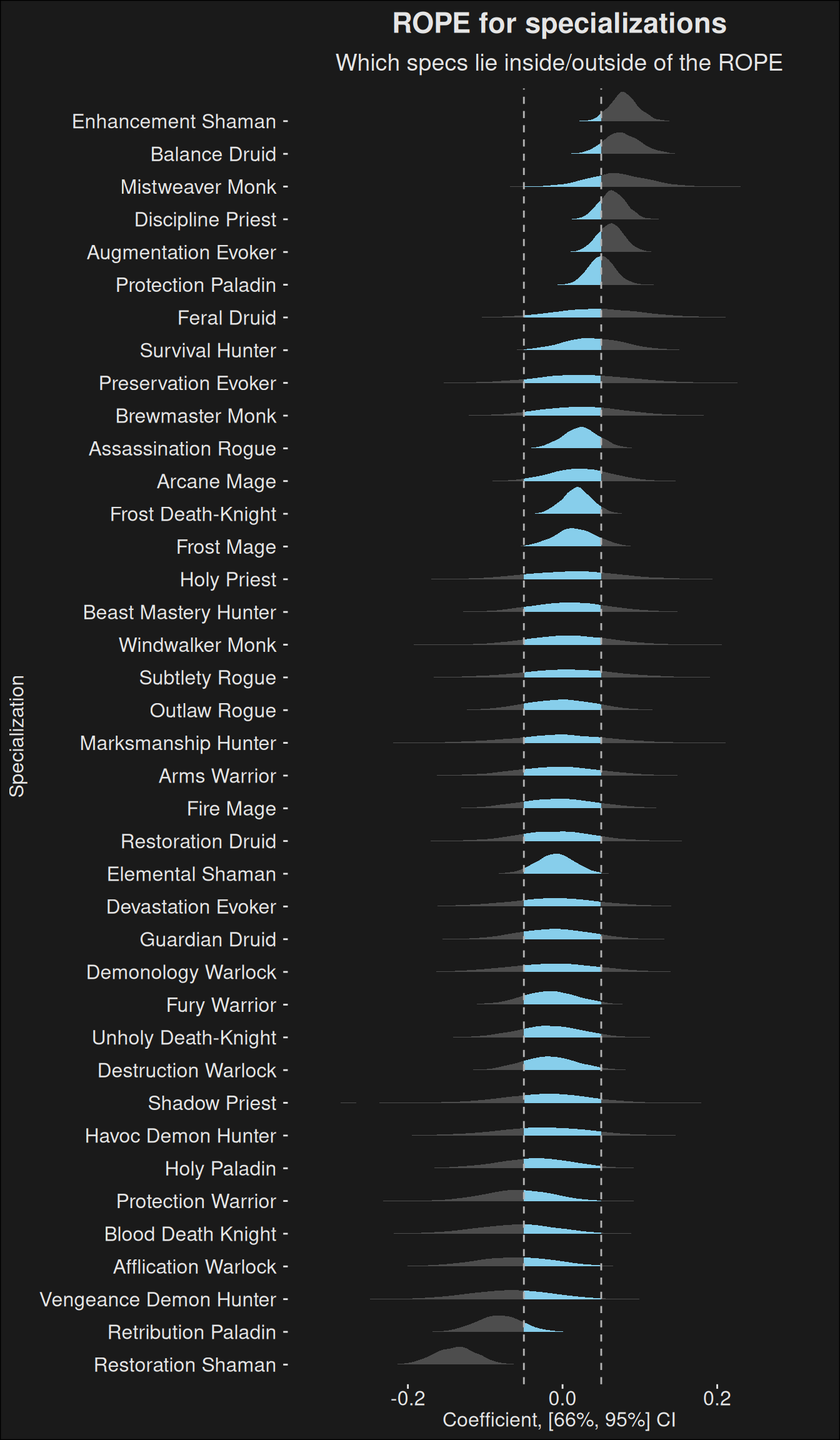
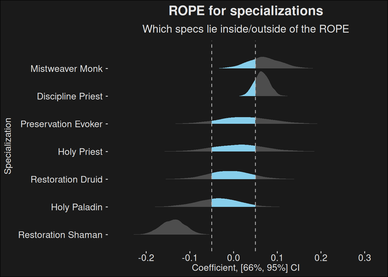
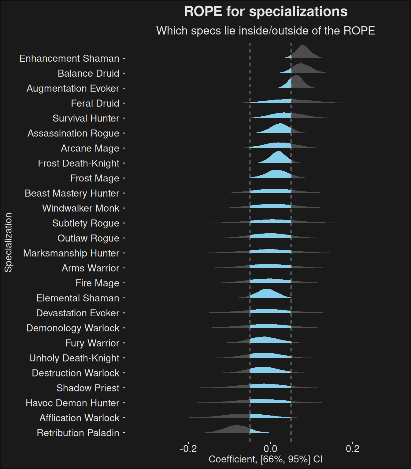
We also have a ROPE-plot for the specializations, which shows which specs lie outside the region of practical equivalence.
Code
spec_rope(fit, data)
Figure 9.2: Specialization strength plotted with a ROPE (Region of Practical Equivalence). If a specialization lies outside the ROPE for most of it’s data, it can be considered over- or underpowered. Specializations falling mostly within the ROPE can be considered equal. Specializations straddling the ROPE boundary is somewhere in between. If a specialization persists being outside the region for several weeks, it might be an indicator the spec needs tuning. The region chosen here \([-0.05, 0.05]\) can be changed depending on the level of balance you want. A smaller interval means more balance, but also more tuning. A larger interval risks we never end up tuning outliers. In practice, you need to keep the ROPE fairly conservative, and only tune if something becomes too much of an outlier.
ROPE-plots give an idea of which specs are so powerful or weak, they have a significant impact on the M+ scores. In short, they have a significant impact on dungeon runs. The band chosen in Figure 9.2 is deliberately somewhat conservative, because there will always be imbalances and rather small imbalances don’t necessarily need tuning.
In the highest of the highest keys, the impact of the specializations have an effect you cannot ignore. In keys slightly below that, the individual player skill can easily compensate for the specialization variance because it is much larger than what you get in specialization contribution. The fact player skill varies that much at the very top suggests it varies even more when you look at the 95th percentile4.
4 TL;DR—Do not use plots like these to select your group compositions in a 1-20 key. You risk skipping over really competent players who are very comfortable on a off-meta specialization because they’ve played it for years. Even as you approach the top 0.1% of players, knowing the player is far more important than what they want to run. Great players can squeeze out power of any specialization.
9.4.4 Roles
Because people like to compare roles, we can extract individual roles into plots of their own. The model is still considering all data points as a whole, but we filter the data down to the roles, so it is easier to compare healers, tanks, and DPS.
9.4.4.1 Healers
A particular strength of a model based on M+ score as a response variable is that it can work correctly with healers. Some other sites5 factors in HPS and DPS of healers in order to gauge strength. This is risky, because neither HPS nor DPS are good indicators of a specializations ability to run high dungeons efficiently (see HPS as a metric and DPS as a metric).
In addition to healers, a model like the one we use can correctly deal with support specializations such as Augmentation Evoker, because it doesn’t rely on correct DPS values to provide a strength estimate.
Furthermore, we can compare the power of different roles to each other: we can place the healer role in relation to the role of tanks and DPS. You can compare, e.g., an Enhancement Shaman to a Discipline Priest if you want. That’s unusual compared to most other models, which treat each role as a separate entity.
Code
role_analysis(fit, data, "healer")
We can also plot the ROPE-plot for healers:
Code
role_rope_analysis(fit, data, "healer")
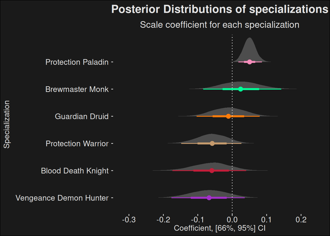
9.4.4.2 Tanks
Tanks are normally particularly hard to rate because their survivability is a large factor of their strength. When tanks die, it often leads to a wipe, so them staying alive is usually more important than the damage output they have. This makes it rather hard to evaluate tanks based on the usual DPS/HPS metrics which the community is fond of. It’s not that HPS/DPS isn’t important, because speed is of the essence to avoid mechanics and also time the dungeon. But for tanks specifically, the factor is lower than for DPS.
Again, by basing the model off of M+ score, we avoid the problem where DPS/HPS of the tank ends up being misinterpreted and given too much weight.
Code
role_analysis(fit, data, "tank")
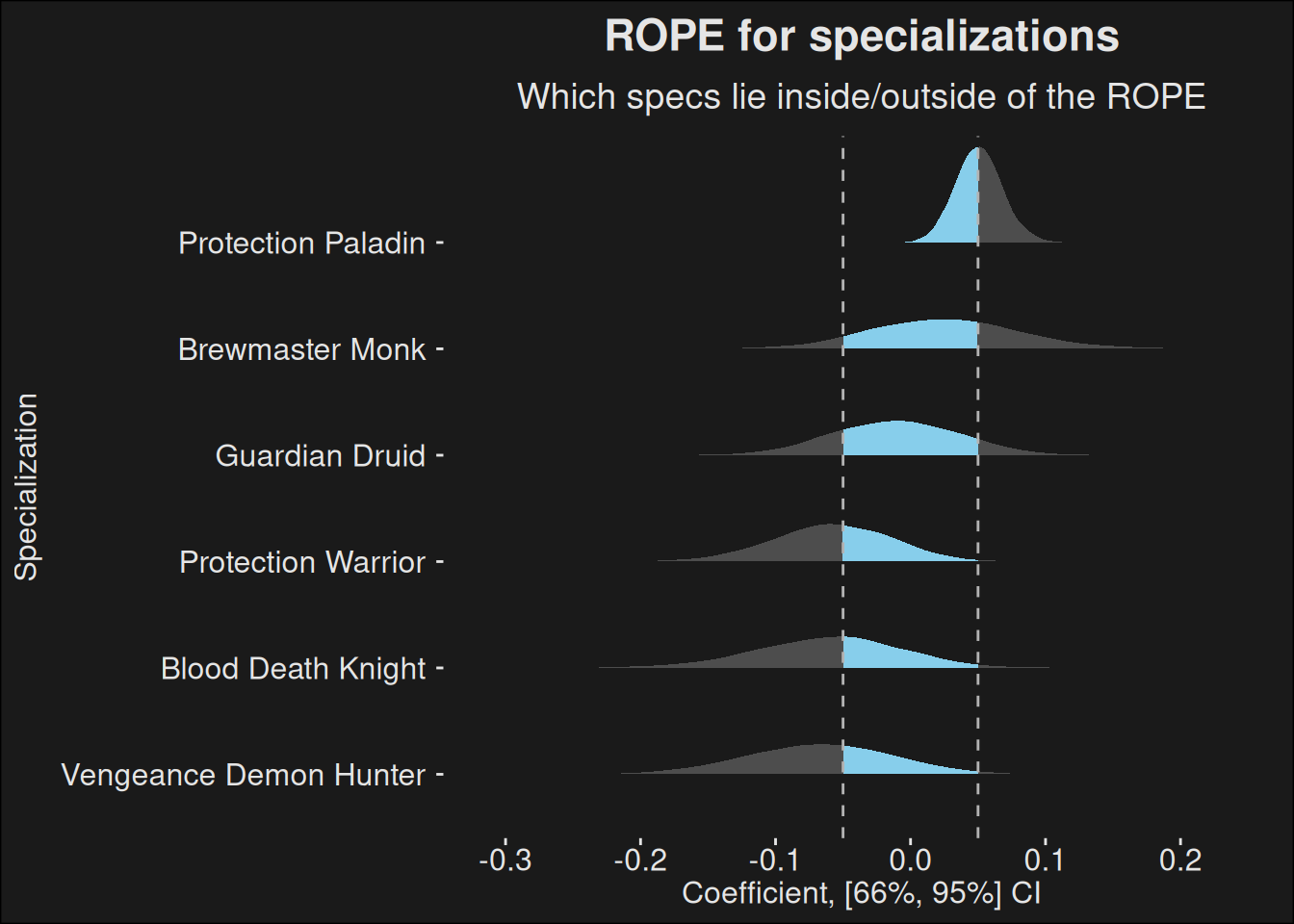
The ROPE-plot for tanks:
Code
role_rope_analysis(fit, data, "tank")
9.4.4.3 DPS
For high level play, the general survivability of a DPS-specialization tends to weigh quite heavily. You need to survive, and you need enough damage to time the key. If a DPS brings additional strong utility, it further helps. This is why these plots might differ from other tier listings where DPS factors in.
Comparing to something like Subcreation, a major difference is that we adjust for dungeon difficulty. Timing a more difficult dungeon is considered better than timing an easy dungeon. After all, it’s the hardest dungeons which tend to explain which specializations are able to survive dangerous mechanics. The other important thing is that a player only counts once, and doesn’t pseudoreplicate. We treat all runs by the player as one input for the specialization, and adjust depending on how consistent the player is.
Code
role_analysis(fit, data, "dps")
Code
role_rope_analysis(fit, data, "dps")
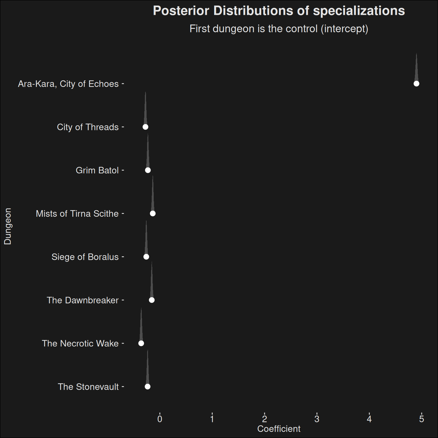
9.4.5 Dungeons
Finally we can plot the dungeons. In the model, this is of less direct interest, but it has indirect value as we use the dungeon difficulty as a scaling factor. This allows the model to counteract a harder dungeon from an easier one, thus evening out the score differences. In turn, it allows us to compare runs across dungeons better, which empowers the data. Hence, we get better estimates of both player skill, and as a result, specialization power.
Code
dungeon_analysis <-function(fit, dat) { fit |>recover_types(dat) |>spread_draws(beta[dungeon]) |>inner_join(dungeon_names, by =c("dungeon"="key")) |>ggplot(aes(y =fct_rev(dungeon.str),x = beta)) +stat_halfeye(fill ="gray30", color ="white") +labs(title ="Posterior Distributions of specializations",subtitle ="First dungeon is the control (intercept)",x ="Coefficient",y ="Dungeon" )}dungeon_analysis(fit, data)
Figure 9.3: The dungeon coefficients of the model, plotted per dungeon. Note that one dungeon is regarded as the intercept-dungeon, and other dungeons are contrasted relative to the intercept-dungeon. The data is used to adjust for the noise dungeon difficulty provides regarding specialization strength. Timing an easy dungeon is not as valuable as timing a hard dungeon. The noise can then be removed, which gives a clearer view of the specializations.
Note that one of the dungoens acts as the intercept, so the other dungeons are contrasted toward this one. That is, their scores are the difference relative to the intercept-dungeon. The reason this is done is for mathematical reasons, where you get computational instability if you try to have a separate intercept. In this model, we are interested in the specializations and not the dungeons, so it is ok if the presentation suffers.