Rows: 6,400
Columns: 9
$ region <fct> eu, eu, eu, eu, eu, eu, eu, eu, eu, eu, eu, eu, eu, …
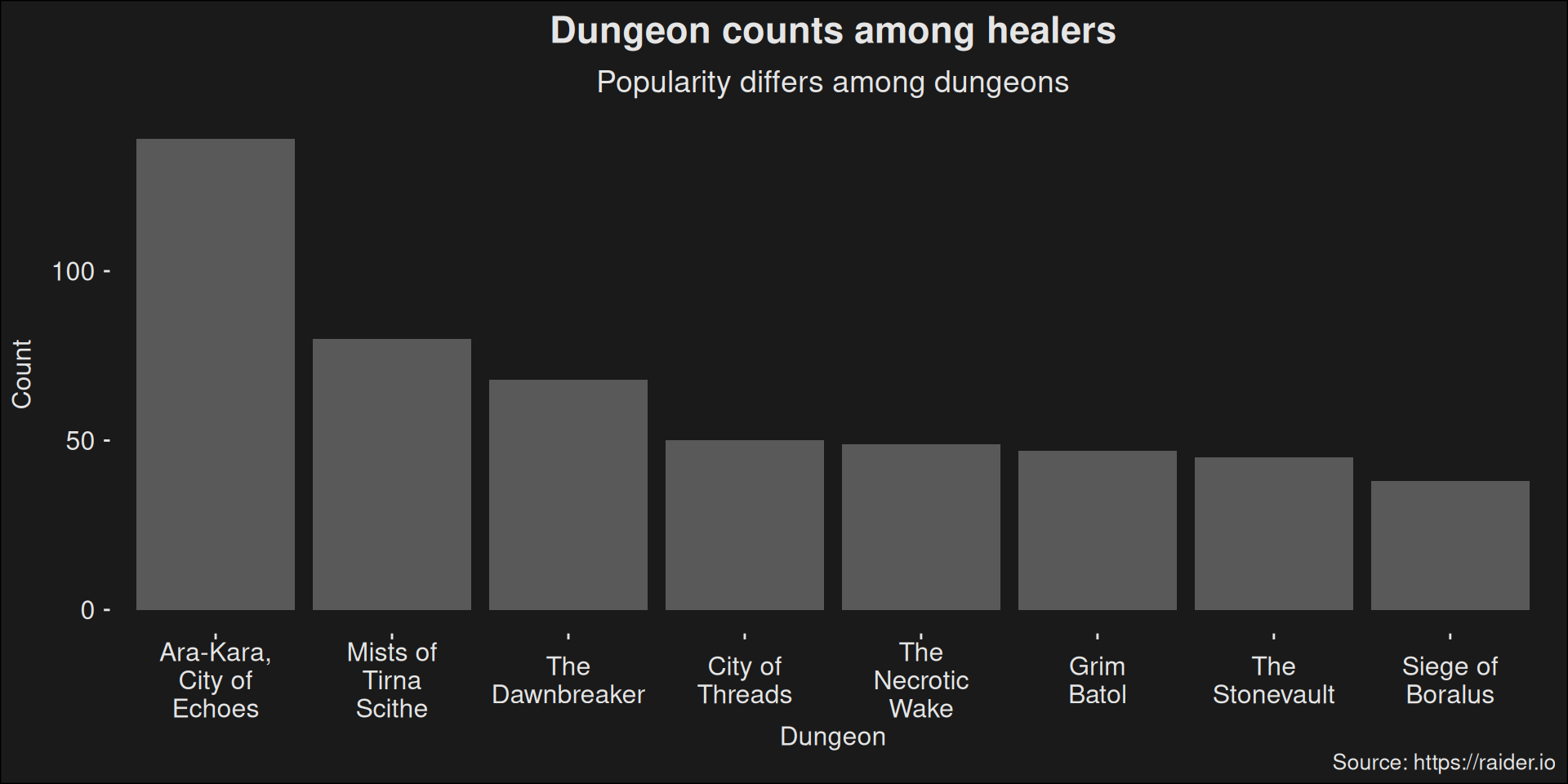
$ dungeon <fct> arakara-city-of-echoes, arakara-city-of-echoes, arak…
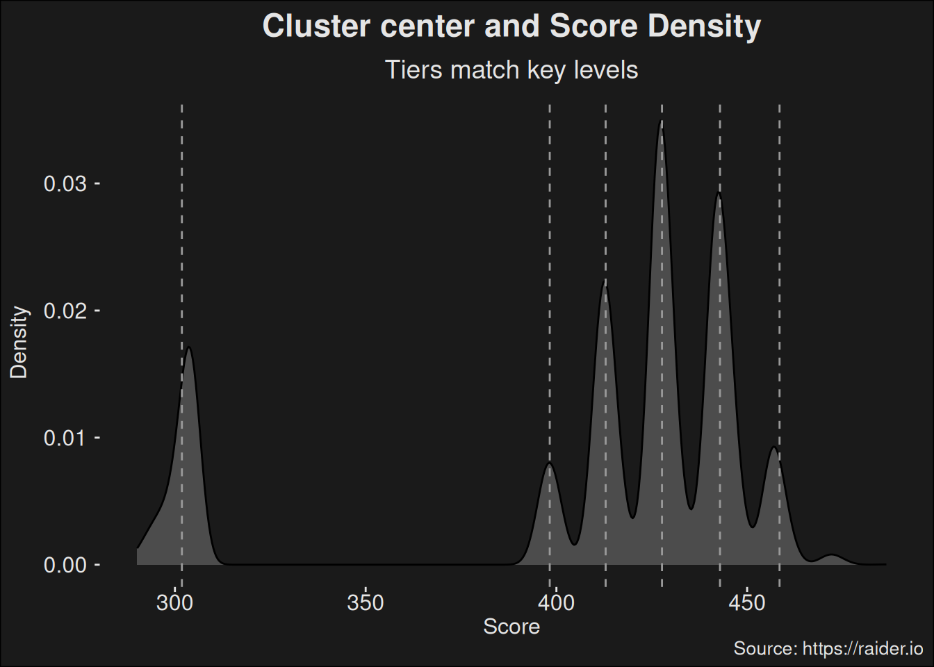
$ key_level <dbl> 20, 19, 19, 19, 19, 19, 19, 19, 19, 19, 19, 19, 19, …
$ score <dbl> 302.6, 475.4, 475.2, 474.1, 473.7, 472.7, 472.7, 472…
$ time_remaining_ms <dbl> -122146, 273021, 261908, 207809, 185420, 137578, 135…
$ group_id <fct> e3de0cddf05856ed8264f4f832a54d84c1a84c68be838fe966c9…
$ tank_id <fct> 197798483, 195435816, 226801834, 195435816, 19779848…
$ healer_id <fct> 168952271, 231776615, 192781776, 231776615, 16895227…
$ dps_id <fct> 82c7313607536e1c73b24d36ecbdfaadb99f5aae06604fe816d1…
Rows: 31,133
Columns: 18
$ region <chr> "eu", "eu", "eu", "eu", "eu", "eu", "eu", "eu", "eu"…
$ dungeon <fct> arakara-city-of-echoes, arakara-city-of-echoes, arak…
$ key_level <int> 20, 20, 20, 20, 20, 19, 19, 19, 19, 19, 19, 19, 19, …
$ score <dbl> 302.6, 302.6, 302.6, 302.6, 302.6, 475.4, 475.4, 475…
$ time_remaining_ms <int> -122146, -122146, -122146, -122146, -122146, 273021,…
$ id <fct> 197798483, 168952271, 232497511, 232493270, 18606320…
$ name <chr> "Yonteaux", "Ihatepriest", "Speedyo", "Elbroiblo", "…
$ role <fct> tank, healer, dps, dps, dps, tank, dps, healer, dps,…
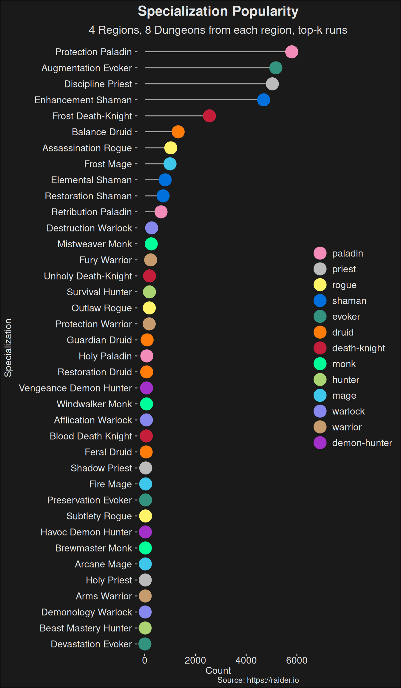
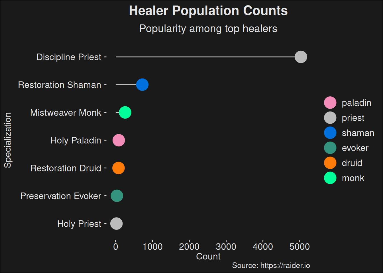
$ class <fct> paladin, priest, rogue, shaman, evoker, paladin, dru…
$ spec <fct> protection, discipline, assassination, enhancement, …
$ has_external <fct> No, Yes, No, No, No, No, No, Yes, No, No, No, Yes, N…
$ has_bloodlust <fct> Yes, Yes, Yes, Yes, Yes, Yes, Yes, Yes, Yes, Yes, Ye…
$ has_resurrection <fct> Yes, Yes, Yes, Yes, Yes, Yes, Yes, Yes, Yes, Yes, Ye…
$ class_spec <fct> paladin_protection, priest_discipline, rogue_assassi…
$ is_ranged <fct> No, Yes, No, No, Yes, No, Yes, Yes, No, Yes, No, Yes…
$ dungeon.abbrev <chr> "AK", "AK", "AK", "AK", "AK", "AK", "AK", "AK", "AK"…
$ dungeon.str <chr> "Ara-Kara, City of Echoes", "Ara-Kara, City of Echoe…
$ region.str <chr> "Europe", "Europe", "Europe", "Europe", "Europe", "E…