This chapter performs data analysis on World of Warcraft specializations. In particular, we are trying to answer the age-old question of which Specialization (spec) you should play if you want the strongest one.
We are trying to breathe some statistics into the debate. The idea is that theories on power/rating can be supported by statistics and data visualization. Some ideas are far easier to reject given data, and other ideas have support. The general layout is that we first analyze the player population as a whole, by looking at players Mythic+ scores across all specializations. In a later chapter, we’ll use the dungeon-based data used by Subcreation as well.
As is common on this site, healers are the initial focus. Once we have a good grasp on the data, we’ll expand the analysis to the other player roles of Tanks and DPS. The analysis is roughly the same, but it is easier to report on a relatively small group of specializations first, rather than get overwhelmed with the full amount of data in the data set1.
1 Don’t put too much into specialization ratings. Your skill and comfort on a given specialization often matter far more than the numbers provided here. In particular, some of these strength-computations are influenced by popularity which puts them on somewhat shaky ground. Use critical thinking.
8.1 Study Design
For the specialization analysis. The first inclination is to use raider.io as a sampling frame. We use the world-wide leaderboards, and pick \(k\) random samples for each specialization we are interested in:
Stratify by spec:
Pick \(k\) random samples from players above 1500 rating.
This is desirable because if there’s some kind of discrepancy between classes, it is likely to show up across the board, and not only at the very top. Also, most people are going to run keys in the range 1-20. We better provide those players with an answer in the range they are playing. By sampling the leaderboards, we also guarantee that each sample is an individual player. That is, we don’t have to control for repeated players in the model. Furthermore, we get data on all dungeons, and can factor in both Tyrannical and Fortifid weeks. All in all, this normalizes a lot of the data.
Another property we get by sampling across a wide player skill level, is we get to “factor in” the difficulty of a spec. If a spec is strong, but also rather difficult to play, it is likely to show up in the data by penalizing the spec. Had we only sampled the best players, they’d be able to play the class well anyway.
Finally, by stratifying over the spec, we avoid popularity problems. Some classes, like Druid, are far more popular than other classes, like Monk. Among healers, for instance, there are roughly 5 times as many Druids than Monks (March 2023). If you don’t stratify, you’ll get roughly 5 times as many druids in the data set, and this will affect a number of computations which are sensitive to popularity.
8.2 Data Import
We’ll repeat the work of doing healers first, then expand into other classes later on by including those at a later point in time.
Code
source('load-players.R')players <- players |>right_join(spec_names, by =c("class_spec"="key"))p_healers <- players |>filter(role =="healer")glimpse(p_healers)
Rows: 2,800
Columns: 11
$ id             <fct> 229469098, 57646788, 110654297, 227912843, 142578441, 1…
$ rank           <int> 12808, 10630, 6032, 17045, 19453, 6413, 20732, 26613, 1…
$ score          <dbl> 2226.37, 2316.07, 2513.39, 2040.07, 1909.24, 2497.07, 1…
$ class          <fct> monk, monk, monk, monk, monk, monk, monk, monk, monk, m…
$ spec           <fct> mistweaver, mistweaver, mistweaver, mistweaver, mistwea…
$ class_spec     <chr> "monk_mistweaver", "monk_mistweaver", "monk_mistweaver"…
$ is_ranged      <fct> No, No, No, No, No, No, No, No, No, No, No, No, No, No,…
$ key.class      <chr> "monk", "monk", "monk", "monk", "monk", "monk", "monk",…
$ key.spec       <chr> "mistweaver", "mistweaver", "mistweaver", "mistweaver",…
$ class_spec.str <chr> "Mistweaver Monk", "Mistweaver Monk", "Mistweaver Monk"…
$ role           <chr> "healer", "healer", "healer", "healer", "healer", "heal…
The data set samples an equal amount from each specialization:
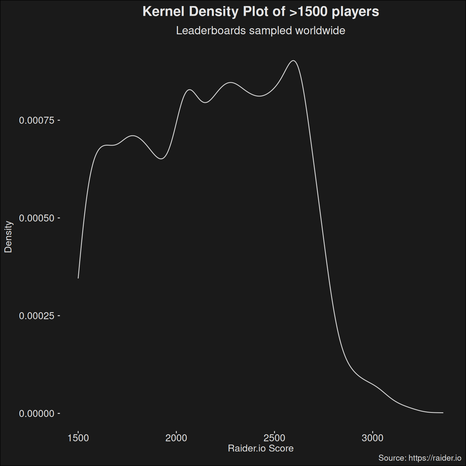
All good data analysis visualizes the data at hand for trends. We begin via a density curve plot. That is, we plot the score obtained on the X-axis, and the so-called kernel density on the Y-axis. A kernel density approximates a probability distribution function, and thus the area under the curve sums to 1. This density tells us the likelihood of observing a value at a given M+ score. The curve will be higher in the score areas with a lot of players, and lower in the area where there are a few players.
Figure 8.1: Kernel density plot of players worldwide having a rating of at least 1500. Each specialization is sampled randomly 400 times among all M+ players. Then all the data points are combined into a large data set which is used for the kernel density plot. Note: in principle, the stratification over specs might change the density curve slightly compared to just sampling randomly in the full data set. However, the following work is interested in the specialization differences, why we stratify.
Plateaus exist at 2000 and 2500 rating. These are breakpoints for the achievements “Keystone Master” and “Keystone Hero”, so it isn’t that surprising people abandon the specialization at that rating score. It would seem people proceed a bit above the 2500 rating mark as well, before they “tap out”. As you get into the higher range, fewer and fewer players are playing at that M+ score. Players above 3000 rating is an exceedingly small part of the player base.
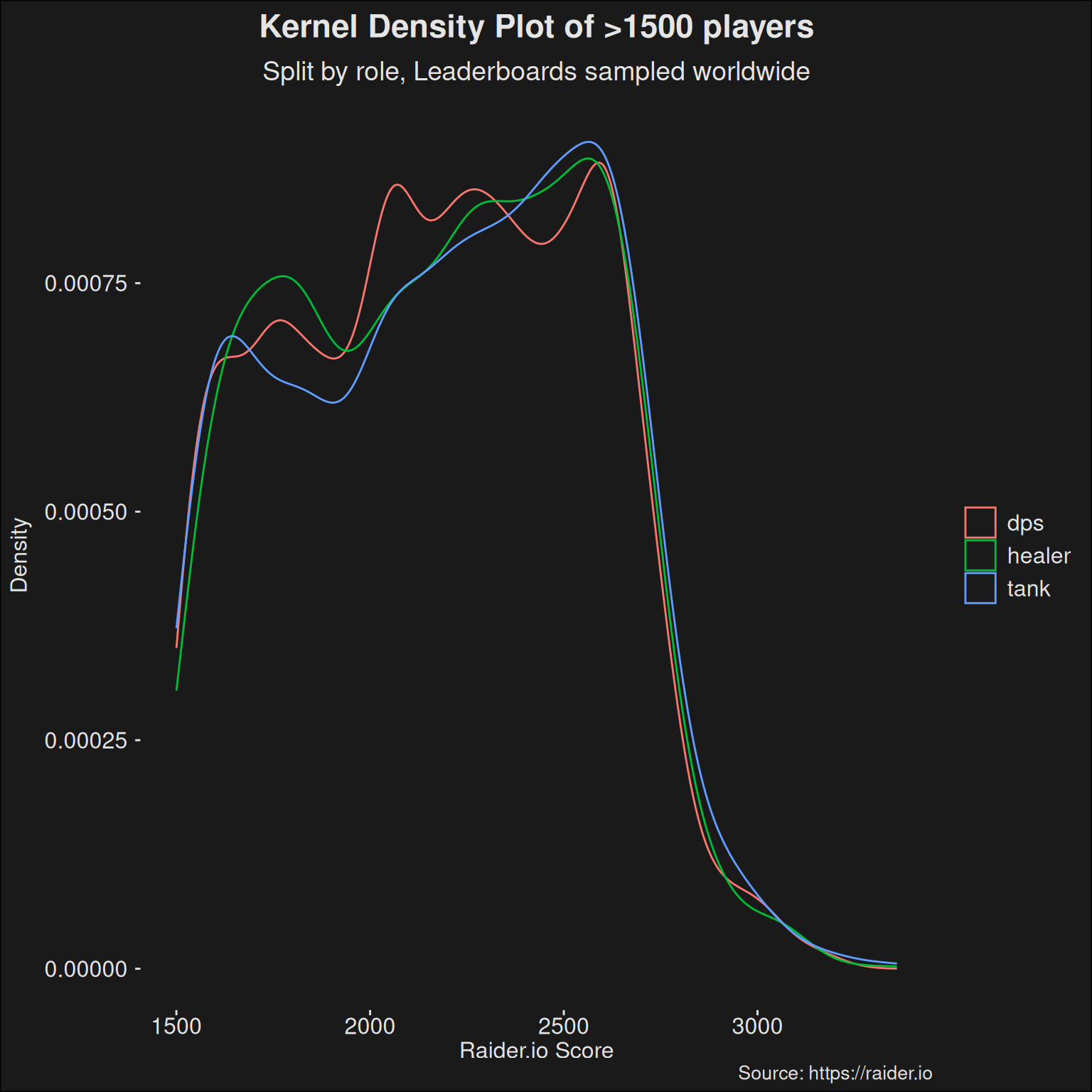
In season 2 of Dragonflight, a talking point has been the lack of healers. We can try a density kernel plot split by role:
Code
players |>ggplot(aes(x = score, color = role)) +geom_density() +scale_y_continuous("Density") +labs(title ="Kernel Density Plot of >1500 players",subtitle ="Split by role, Leaderboards sampled worldwide",x ="Raider.io Score",caption ="Source: https://raider.io" )
Kernel density plot of players, split by role. Some roles have an easier time pushing to higher key levels than others. The guess is this is mostly because some roles generally run more keys over a time window, so they’ll typically get to higher key levels pretty easily. This then affects the scores obtainable by those roles.
While it might be harder to play a healer, it is not immediately reflected in the IO levels the roles can reach. It is rather DPS which has a harder time, likely because getting into groups as a DPS is more difficult.
8.3.1 Popularity
Specialization popularity has an effect on the results provided here. The reason you have so many specializations close to 0 rating is because people bring their alts into M+ to get items in the vault. The active players are lower because you might have several alts for each main.
Hence, if a lot of people are active on a given specialization, that activity will improve their representation over the full spectrum of M+ scores, and alts will be sitting at lower ratings. This injects some noise in the data when we are sampling in all the possible players.
Popularity is a combination of many factors:
Is the spec fun to play? Some rotations are just far more fun and rewarding to play than others. You can have an incredibly strong spec that’s boring to play, and this will have an effect.
Is the spec strong? Stronger specs sees more play, because there’s a group of people who likes to chase whatever has the most power each season. They like to re-roll into the current strongest spec, and are more interested in chasing higher scores than living a given class fantasy.
Is it easy to play? Some specs have low skill floors, and doing decently on them doesn’t take much work.
Is it hard to play? Some specs have high skill ceilings, which means you need to be familiar with the spec to squeeze out the full value.
As stated elsewhere on this site, the community of players are “figuring out” a spec, and by doing so, they increase the power it has. Thus, popularity, community, and power are interlinked and not something you can separate entirely.
8.3.2 Healers
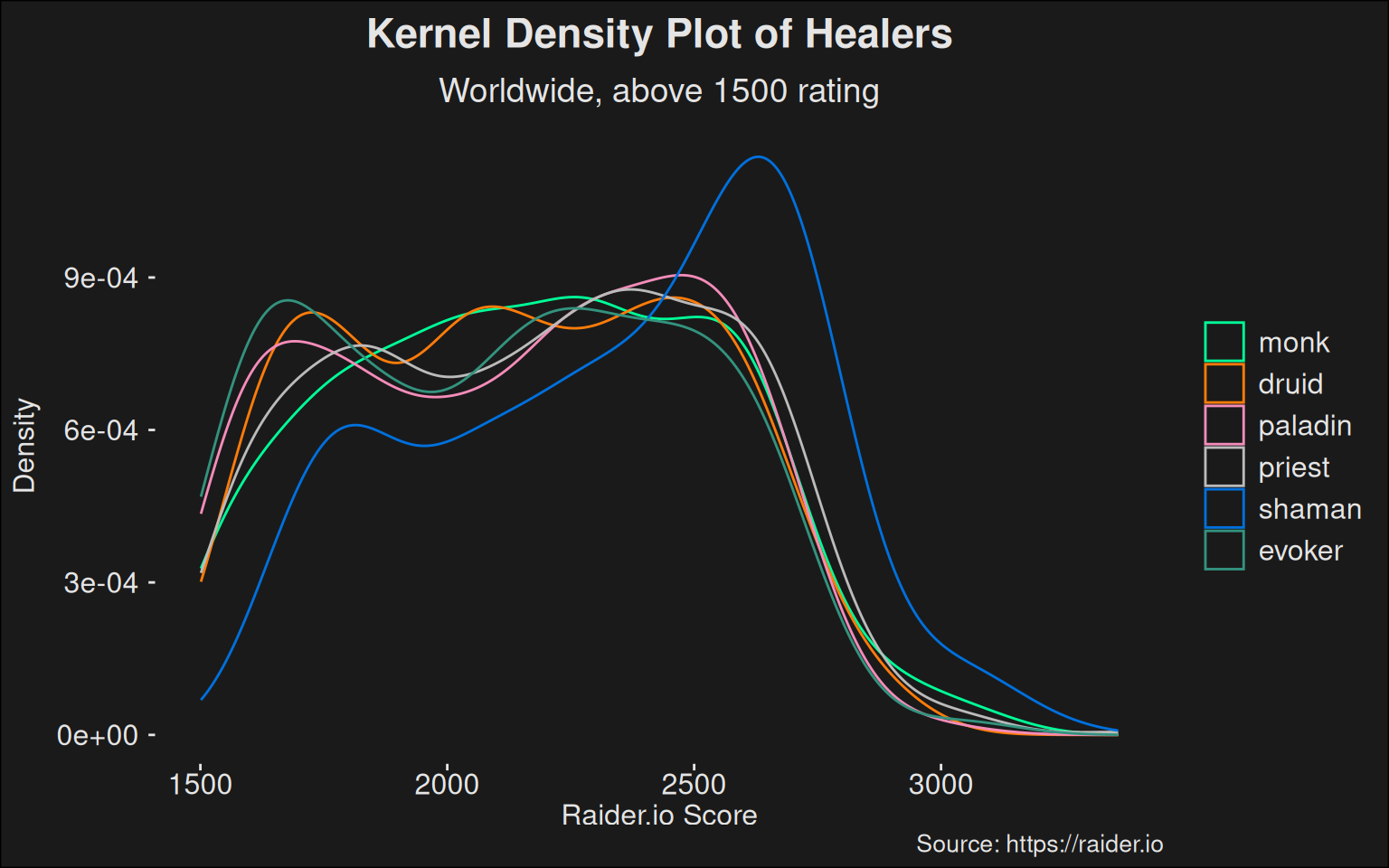
If we focus on healers, we get the following kernel density plot:
Figure 8.2: Kernel density plot of healers. Note that the two priest-specs are combined into a single group here, mainly to avoid overplotting in an already noisy plot.
I think there’s a lot of valuable information in sampling over a wide skill range. Some trends can only be fully appreciated if we look at the full data set.
People like to look at the top, because they assume that is where a spec is being squeezed to its full potential. But I claim there are important indicators at all skill levels. Later on in this chapter, we’ll have a look at the top players, but for now, we are going to work with data above 1500 rating2.
2 The choice of 1500 rating is somewhat arbitrary. It’s high enough to cut a lot of noise at the bottom, yet low enough most people who make an effort can grind there relatively easily. For a wider data set, we want relatively unskilled people in the population.
When we look at the density curves, it’s pretty obvious data isn’t normally distributed. We’d like to build a model for this data, but the standard linear regression model (for categorical data) won’t work. However, a generalized linear model may.
Here’s the overarching idea: we’d like to use linear models if possible, because our linear algebra toolbox in math is really good. We know a lot about linear relationships and we can utilize the large toolbox to our advantage. But the data isn’t linear. One possible way around this problem is to transform data before we work with it. If we can transform data so it becomes linear, then we can use our linear algebra hammer.
However, another possible way is to insert a link-function in our linear model. The link-function acts like an optical lens of sorts. It bends the “light” which originates from the data so it becomes linear on the other side of the lens. This allows our linear hammer to work but on data which has not been transformed beforehand.
You may think these two methods are exactly the same, but there are some subtle details in which they differ. A transformation will also transform the error (noise) of the model, whereas a link-function won’t.
As a whole we call the models Generalized Linear Models (GLMs). GLMs allow the response variable (here: score) to be distributed in a way that isn’t normal. They allow distributions from the so-called exponential family. Typical examples are the normal and poisson distributions. Because of the skew in the data, we can choose to model scores as a GLM where the family is a Gamma distribution, and the link-function is \(\log(\cdot)\).
We know it won’t be a perfect fit. In the words of George Box,
All models are wrong, but some are useful
In particular, we know there are additional modalities in the data. At rating levels \(2000\) and \(2500\) we have the achievements Keystone Master and Keystone Hero respectively. Also, some people regard a rating of \(3000\) a nice round number where they are happy with their performance. Thus, we’d expect the model to be wrong, because we aren’t going to model these interactions.
Your friendly data-exploring Mechagnome is more of a Bayesian gnome than a classical statistics gnome. Hence, all of this will be done via Bayesian modeling in stan. We can implement our model as a small program:
data { int<lower=1> N; // total number of observations vector[N] y; // response variable int<lower=1> K; // number of population-level effects matrix[N, K] X; // population-level design matrix}transformed data { // matrices for QR decomposition matrix[N, K] XQ; matrix[K, K] XR; matrix[K, K] XR_inv; // compute and scale QR decomposition XQ = qr_thin_Q(X) * sqrt(N - 1); XR = qr_thin_R(X) / sqrt(N - 1); XR_inv = inverse(XR);}parameters { real tau; // mean of bQ real<lower=0> sigma; // coefficient variance parameter vector[K] bQ; // regression coefficients at QR scale real<lower=0> shape; // shape parameter}transformed parameters { real lprior = 0; // prior contributions to the log posterior lprior += normal_lpdf(tau | 0, 5); lprior += cauchy_lpdf(sigma | 0, 5); lprior += normal_lpdf(bQ | tau, sigma); lprior += cauchy_lpdf(shape | 0, 2.5);}model { // likelihood including constants // initialize linear predictor term vector[N] mu = rep_vector(0.0, N); mu += XQ * bQ; mu = exp(mu); target += gamma_lpdf(y | shape, shape ./ mu); // priors including constants target += lprior;}generated quantities { array[N] real y_rep; // obtain the actual coefficients vector[K] b = XR_inv * bQ; // replicated samples for checking y_rep = gamma_rng(shape, shape ./ exp(X * b));}
When doing Bayesian inference, we need to state our prior belief. That is, we need to state what we know about player population before we observe the data. Bayesian frameworks then compute a posterior belief, which is based on the model, the prior, and the data we observed. Generally, the more information we have beforehand, the better our posterior estimates will be.
One might think we should use a prior which is highly non-informative. That is, the prior imposes as little information as possible. This would give more weight to the data and have it stand on its own. But I think this is wrong. If balance in specializations gets too much out of whack, then Blizzard is going to intervene. This suggests there’s a limit to the madness of how far apart we think the specializations are. Previous experience shows a value around \(5\) is quite likely. So we’ll set up our prior to be a normal distribution at \(5\) with an SD of \(2.5\).
In any case, we have so much data that if our prior guess is only slightly correct, the data will eventually overpower the incorrect prior, and provide a posterior based mostly on the data.
Informative priors helps the sampler inside stan by giving it good starting points and ensuring the quality of the samples is high.
Running this model requires us to pass data to it in order to get a fit. We can set up this data so it fits as input to the program.
With the input specified, we can run our stan-program on it. Here, we run the default of 4 MCMC chains, and 2000 iterations, where the first 1000 is used for warmup.
Code
iter <-2000mod <-cmdstan_model("models/specializations.stan")res <- mod$sample(data = player_data,chains =4,parallel_chains =4,refresh =200)
fit <- cmdstanr::as_cmdstan_fit(res$output_files())
Our model is predicting score (the outcome or response) based on the specialization (the predictor). The idea is that we think each specializations scores are Gamma-distributed. If we draw a random player from a specialization, we are far more likely to get a player in the \(1500\text{--}1700\) score range than in the \(3000\text{--}3200\) range. Player count tapers off as we go to higher and higher rating.
But our model will look at each specialization in isolation. It might be there are slight variations in the curves between specs. Analyzing those curve differences is a measure of spec strength. If we can capture this difference, we have a sound argument as to which specialization is the strongest. The crux of this is that the common individual player skill is largely picked up by the Gamma-distribution curve. What’s left is then the difference between specializations, without considering the typical player skill.
This model is wrong insofar some specializations will have highly skilled players flock to them moreso than others. And they might be able to skew the numbers. But we are going to ground this here, by using all players. This makes highly skilled players less of an issue since there are few of them.
A posterior predictive check uses the model in a sort-of backwards direction. We use the model to draw some typical examples of data, by using it as a way to predict. These are forgeries, but they do something useful. If we compare them to the original data, we can get a glance at how good our model fit is. If it is way off, we know it is pretty bad. If it is somewhat agreeing, the model might still be bad, but at least it isn’t violating predictive power.
We have done posterior predictive checks on this model, and the fit is rather good, so we’ll go ahead.
8.3.2.1 Full data fit
In a divergence from Subcreation, we fit all specializations at once. Subcreation fits data to each independent role, and further fits data for DPS into groups of “ranged” and “melee”. By doing a fit on all groups at once, we save some computation, and we arguably get a better model since it is being built on more observed data. In our case, the Gamma-distribution has two parameters, \(\alpha\) and \(\beta\). The first one, commonly called the “shape”, it inferred by use of the full data set. The second parameter, commonly called the “rate”, is what we allow to vary between specs. By factoring in all specs for the shape parameter, we get an estimate of it with more data.
Once we have fitted all of the observed data, we can recover the data from healers pretty easily:
Code
fit |>recover_types(data) |>spread_draws(b[class_spec]) |>inner_join(spec_names, by =c("class_spec"="key")) |>filter(role =="healer") |>ggplot(aes(y =fct_rev(class_spec.str), x = b, color = key.class)) +stat_dotsinterval(quantiles =100) +scale_color_manual(values = wow_colors) +scale_fill_manual(values = wow_colors) +labs(title ="Posterior >1500 rating Healer Power (median)",subtitle ="Bands: 66% and 95% of the distribution",y ="Specialization",x ="Coefficient" )
Warning: No shared levels found between `names(values)` of the manual scale and the
data's fill values.
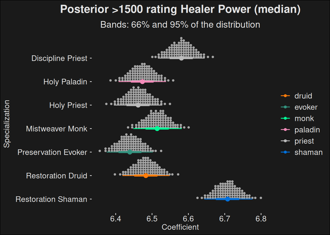
Figure 8.3: Plot of estimated healer power computed as a posterior distribution from raider.io leaderboard data. For each healer, the coefficient encodes the dropoff curve for each specialization, with higher values being a flatter curve with more players at higher levels. The distribution explains the uncertainty for the estimates, with a wider distribution meaning more uncertainty for the given specialization. Due to the number of samples being roughly the same, the distributions tend to have roughly the same amount of uncertainty.
For a more in-depth description of the coefficient, see the section on (leaderboards-top-players?) where there is a precise description.
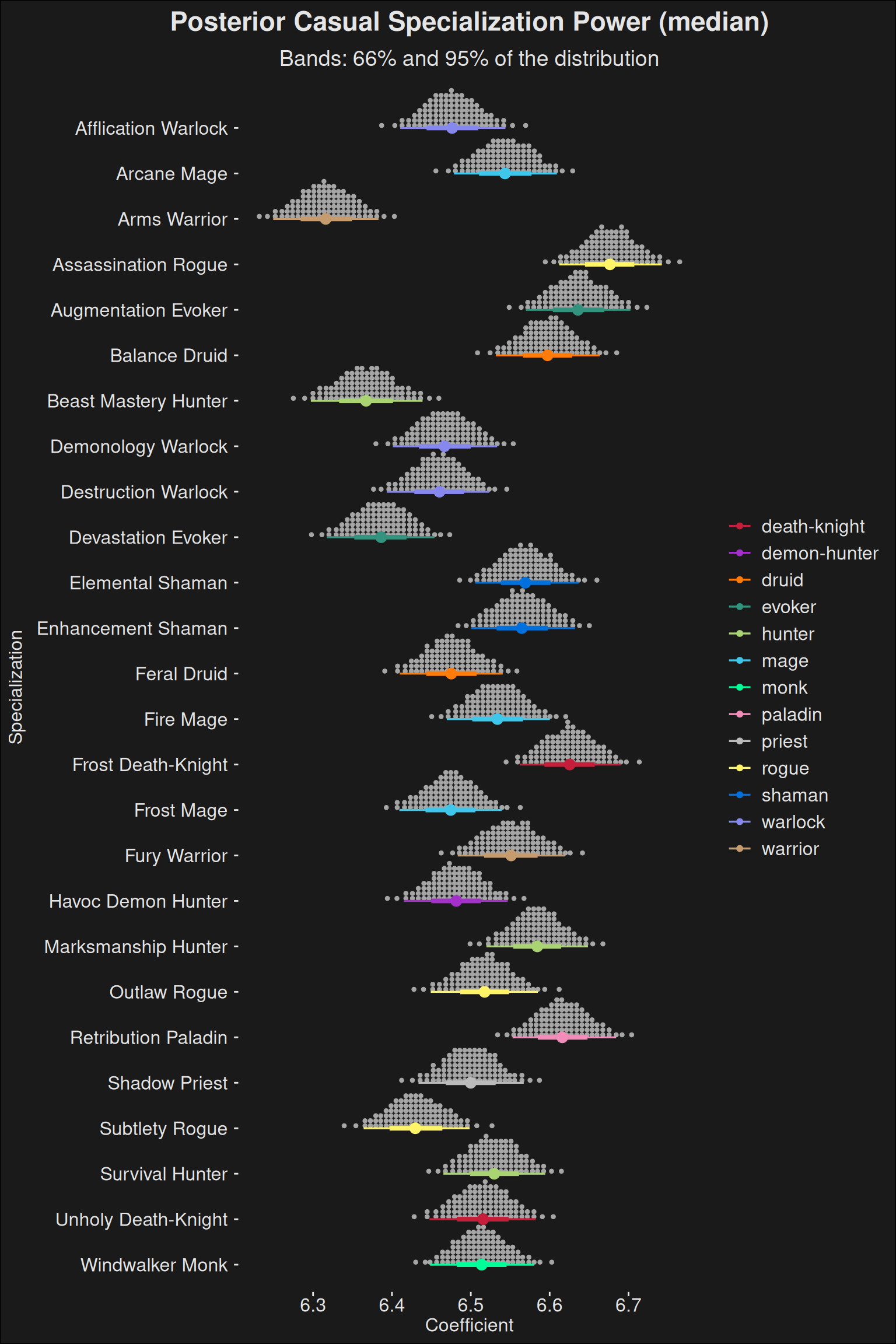
In this plot, dots are a quantization of observations, with 100 dots. Their distribution is the outcome of the “rate” coefficient from the different specs. The colored dot marks the median of that distribution, which you would use if you were to give a point estimate for each spec. The interval bands are credible intervals which tells you where 66% and 95% of the distribution falls. The idea is that it captures the uncertainty of our estimate, with a wider band meaning we are less certain. Also, if these bands overlap, it might not be the case that one spec is stronger than the other, as we can’t be certain.
8.3.3 Tanks
Having handled healers in detail, the following presents data with less explanation and more discussion.
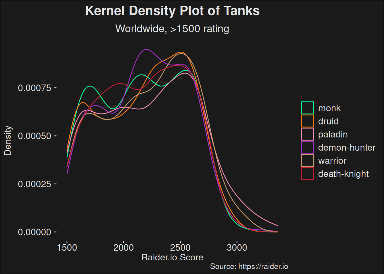
Density plot of tanks above 1500 rating. This plot shows the distribution of tanks over a wide skill range. Note that due to density estimation, the plot is not accurate close to 1500 rating.
In general, a flatter curve represents a stronger specialization. This is because more of the density mass is shifted to the higher scores, so more players managed to achieve a higher score with the specialization.
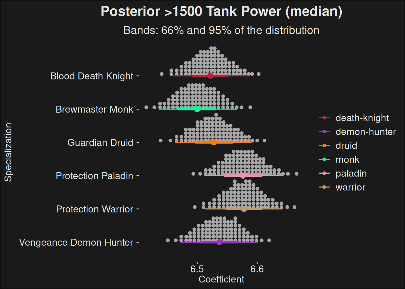
We can extract the posterior medians for tanks as well. This is arguably the most interesting part because it gives you a view of the relative specialization strength over the different options.
Note if there’s a large overlap in the 95% CI, then the specs are for all senses and purposes equal. There’s simply too much uncertainty in the data to declare a clear winner.
Code
fit |>recover_types(data) |>spread_draws(b[class_spec]) |>inner_join(spec_names, by =c("class_spec"="key")) |>filter(role =="tank") |>ggplot(aes(y =fct_rev(class_spec.str), x = b, color = key.class)) +stat_dotsinterval(quantiles =100) +scale_color_manual(values = wow_colors) +scale_fill_manual(values = wow_colors) +labs(title ="Posterior >1500 Tank Power (median)",subtitle ="Bands: 66% and 95% of the distribution",y ="Specialization",x ="Coefficient" )
Warning: No shared levels found between `names(values)` of the manual scale and the
data's fill values.
Posterior rate computations for tanks. The coefficient is a measure of how flat the density curves are. Tanks with more high-rating longevity is considered stronger than tanks with less.
8.3.4 DPS
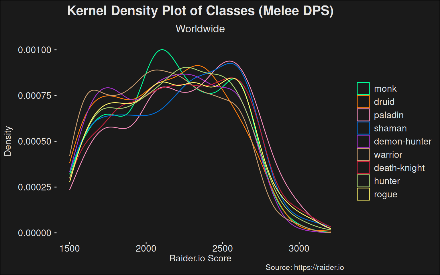
In some of the following density plots, we’ve coalesced all specs for a given class into the same line. While this isn’t ideal, it prevents overplotting and still gives you a class-centered view of the density. Arguably, this is okay because players within (pure) DPS classes tend to be able to switch to whichever spec is the strongest in the game, currently. The ease of swapping penalizes weak specs further and advantages strong specs likewise.
fit |>recover_types(data) |>spread_draws(b[class_spec]) |>inner_join(spec_names, by =c("class_spec"="key")) |>filter(role =="dps") |>ggplot(aes(y =fct_rev(class_spec.str), x = b, color = key.class)) +stat_dotsinterval(quantiles =100) +scale_color_manual(values = wow_colors) +scale_fill_manual(values = wow_colors) +labs(title ="Posterior Casual Specialization Power (median)",subtitle ="Bands: 66% and 95% of the distribution",y ="Specialization",x ="Coefficient" )
Warning: No shared levels found between `names(values)` of the manual scale and the
data's fill values.
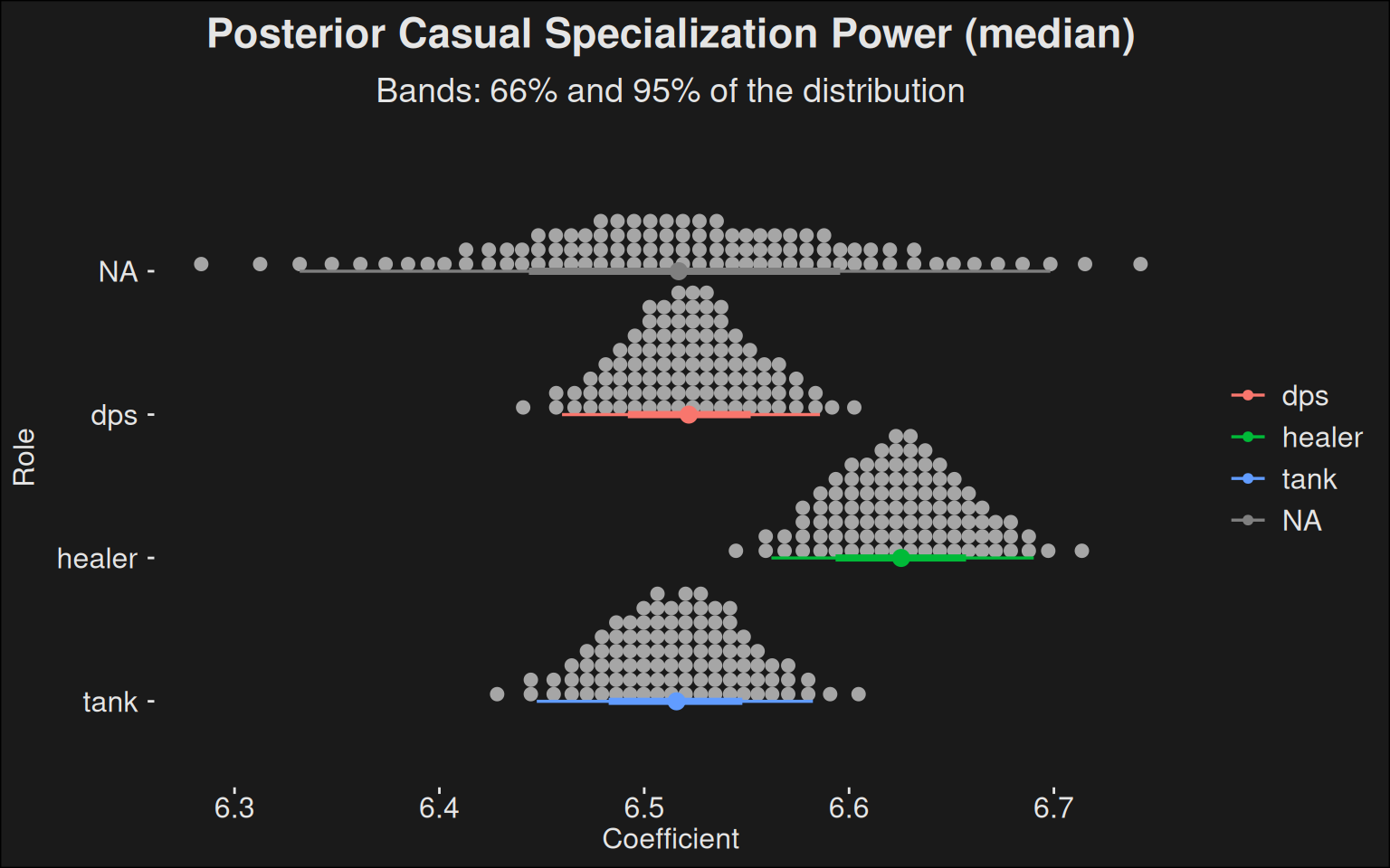
8.3.5 Roles
Analysis of roles could be interesting. Rather than working with each individual spec, we could take a look at the rating of each role against each other.
fir <- cmdstanr::as_cmdstan_fit(res$output_files())
Code
fit |>recover_types(data) |>spread_draws(b[role]) |>ggplot(aes(y =fct_rev(role), x = b, color = role)) +stat_dotsinterval(quantiles =100) +labs(title ="Posterior Casual Specialization Power (median)",subtitle ="Bands: 66% and 95% of the distribution",y ="Role",x ="Coefficient" )
8.4 Top Players
Having analyzed the casual player base, we turn our focus toward the top players. For each specialization, we find players with more than \(2700\) in score, and sample within these. This gives us a view of what the better players are doing, and if they have any kind of different behavior.
Code
players_topk <- players_topk |>right_join(spec_names, by =c("class_spec"="key"))p_healers_topk <- players_topk |>filter(role =="healer")
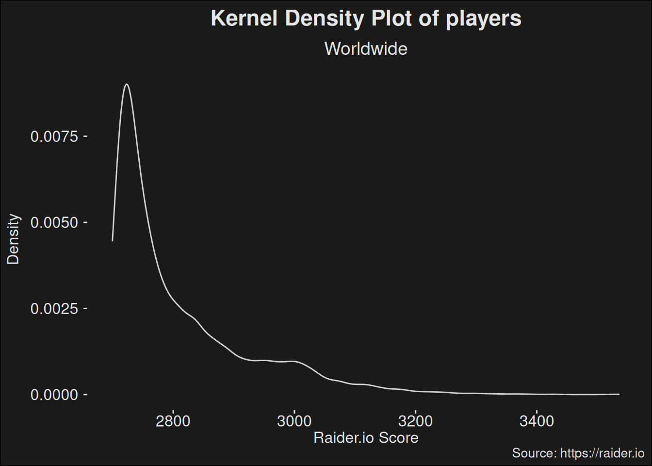
The count is the same as in the case of the casual player base:
players_topk |>ggplot(aes(x = score)) +geom_density(color="lightgray") +scale_y_continuous("Density") +labs(title ="Kernel Density Plot of players",subtitle ="Worldwide",x ="Raider.io Score",caption ="Source: https://raider.io" )
The cutoff choice of \(2700\) avoids the plateaus from Keystone Hero and Keystone Master. Hence, we get a curve which is closer to a typical Gamma distribution.
8.4.1 M+ Score
If we sample a random player, among the high-scoring players, they’ll be somewhere in the above distribution. They are far more likely to be at the lower end than the higher end. That is to be expected. We think that as we increase Mythic+ rating, fewer and fewer players are able to keep up and they “decay” from the population. This view means players are likely part of a Poisson process, and it justifies our use of a Gamma distribution to model the players.
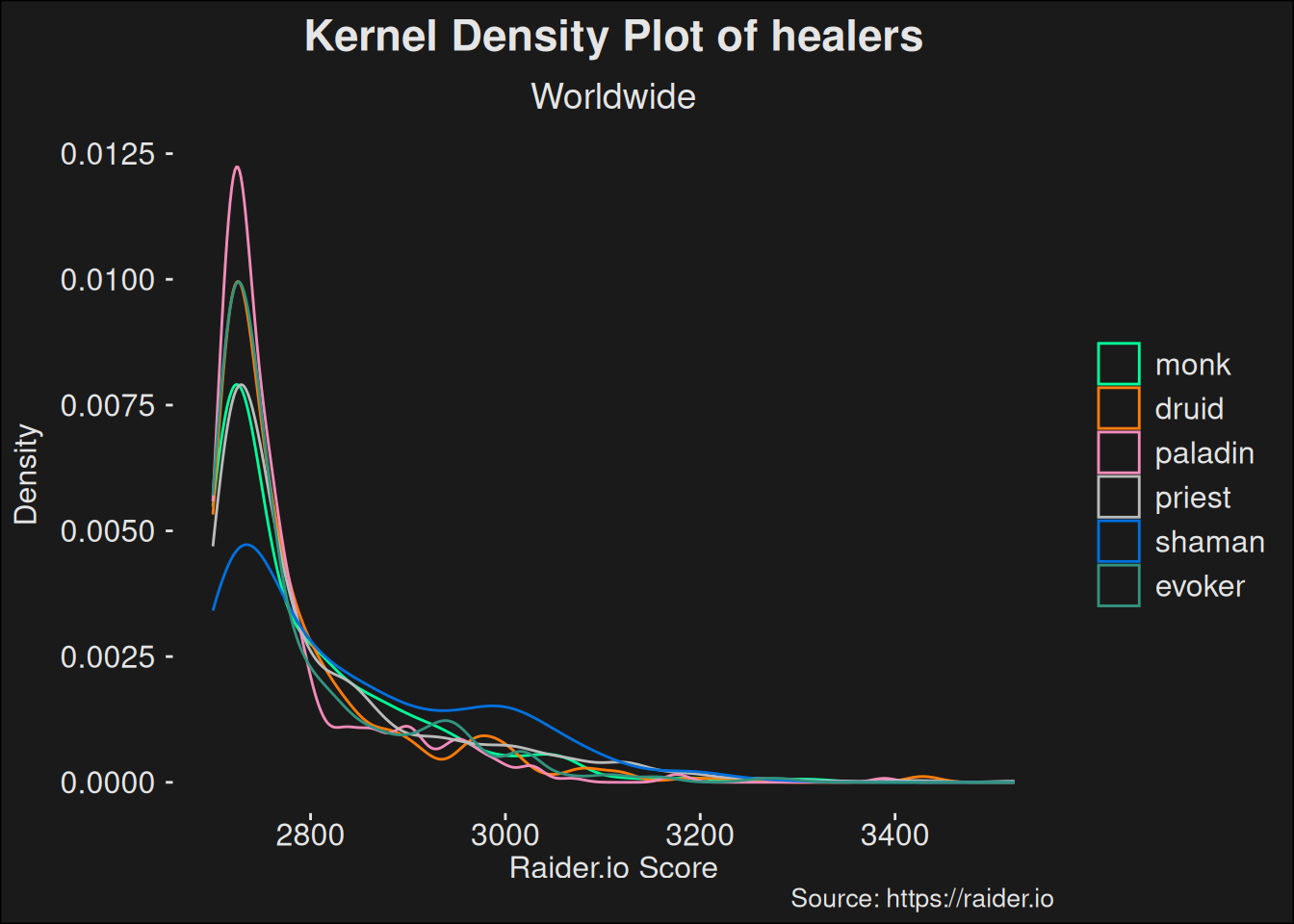
Code
players_topk |>filter(role =="healer") |>ggplot(aes(x = score, color = class)) +geom_density() +scale_color_manual(values = wow_colors) +scale_y_continuous("Density") +labs(title ="Kernel Density Plot of healers",subtitle ="Worldwide",x ="Raider.io Score",caption ="Source: https://raider.io" )
We can construct a model by analyzing the high-scoring players. First, we want to rescale the scores, such that a base score of 2700 is at 0. This centering of the score will make a Gamma distribution applicable in our generalized linear model.
Next, we want to predict the scaled score by means of the specialization being played. This gives us an estimation for each of the specialization categories, which in turn allows us to look for differences among the specializations.
fit <- cmdstanr::as_cmdstan_fit(res$output_files())
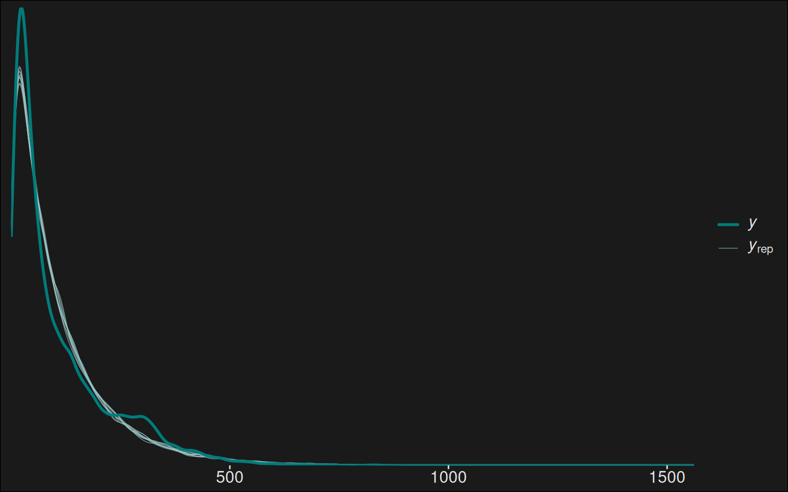
Again, we’d like a posterior predictive check. That is, we are going to simulate a number of runs via the model and compare those simulations to the actual data. In a sense, we are going backwards: we fitted a model. Now we use the model to generate forged data, which we can then compare to the real data.
We’d like these draws from the model to be close to the data we collected. Because that would imply our model is rather good at prediction.
We did this for the model, and the fit looks rather good:
Code
y <- data_top$score_scaledyrep <- fit$draws("y_rep", format ="matrix")color_scheme_set("teal")ppc_dens_overlay(y, yrep[1:10, ])
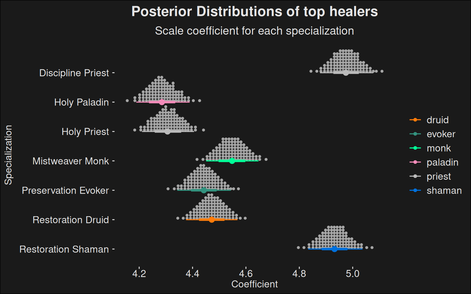
Code
fit |>recover_types(data_top) |>spread_draws(b[class_spec]) |>inner_join(spec_names, by =c("class_spec"="key")) |>filter(role =="healer") |>ggplot(aes(y =fct_rev(class_spec.str), x = b, color = key.class)) +stat_dotsinterval(quantiles =100) +scale_color_manual(values = wow_colors) +scale_fill_manual(values = wow_colors) +labs(title ="Posterior Distributions of top healers",subtitle ="Scale coefficient for each specialization",x ="Coefficient",y ="Specialization" )
Warning: No shared levels found between `names(values)` of the manual scale and the
data's fill values.
In the plot, we have a coefficient value on the X-axis. To explain this coefficient, we need a slight detour: a couple of different characterizations of the Gamma-distribution exists, so we need to be precise in what version we are using. The one used by stan is the typical bayesian formulation where we have a shape parameter \(\alpha\) and a rate parameter \(\beta\). The formulation is
We learn the parameter \(\alpha\) from the data we observe. In the Gamma distribution, we have the mean \(\mu = \frac{alpha}{beta}\). Rearranging this a bit yields \(\beta = \frac{\alpha}{\mu}\), and this is what we plug into the gamma distribution. That is, we estimate a mean \(\mu\) in our stan-program. Because we use a log-link, we compute \(\exp{(\mu{})}\) and use this in our gamma distribution. The parametrization around \(\mu\) is nicer to work with in practice. For instance, we can compute the original score via a function \(g(x) = e^{x} + 2700\), for a coefficient \(x\).
Lower coefficient numbers are more like one big spiky mountain, whereas higher numbers correspond to a rolling hill. The higher the coefficient, the more the specializations M+ scores are spread out.
Compared to the more casual coefficients, we see a clear difference. Specializations which are usually deemed difficult to play go from being fairly low to being fairly high. Higher numbers is an indicator that we are dealing with a stronger specialization, as most of the players at the top level tend to achieve higher scores.
One might surmise if some of this isn’t just due to a popularity among the skilled players. That is, if a coefficient is larger, it’s because the skilled players enjoy said specialization more. This will always be impossible to split given this data. In fact, spec power and player skill are likely to interact. As a whole, the player base of a spec will improve their skill over time. This means it gets more powerful as more people learn how to play it well. And this can lead to the spec becoming so powerful it will need intervention by Blizzard. Likewise, a spec which isn’t figured out yet, might need intervention as well to bring it into balance with the other options.
Our model computes the distribution of player skill as a whole. And then we look if the specs deviates from each other, and by how much. A strong deviation means the spec is either more powerful, or the players are generally better at the spec.
In a sense, the whole question of balance requires you to factor in the players. The community is vibrant and dynamic. It changes all the time. People master their ability in the game. This changes the relative power of a specializations over time. And indeed, the fact there’s a difference between the top and the more casual data could indicate that power cannot be understood in isolation. Indeed it’s the interaction between a players skill and the specializations power which ends up having an effect on the final M+ score.
In short: you sometimes nerf because the player base got too good at playing a given specialization. This can happen even if the nerf is only applicable among the top players, or among the more casual players. It also means nerfs and buffs have to be done with caution. If the player base figured out a spec, it should still have viability in the game after adjustment. Hence, many small adjustments are preferred to large swings in power. Also, there’s no reason to upheave the ordering of specs too much, balance wise. You just want them to be closer to each other.
8.4.1.1 Balance Window
We should ask if the balance window is rather small or large. The mean of a gamma distribution is \(\alpha{} / \beta{}\). In our case, a score of \(4.6\) then amounts to \(\alpha / (\alpha / e^{4.6}) + 2700 = 2799\) because the \(\alpha\) will cancel out, and a score of \(5.15\) amounts to \(e^{5.15} + 2700 = 2872\). That means the difference between the worst and best performing spec is about \(73\) M+ scoring points in the above plot.
A rough rule is to divide this by \(10\) to get a ballpark estimate per dungeon. This ballpark estimate also accounts for Tyrannical/Fortified weeks. So it’s about \(7.3\) M+ score points per dungeon. Is that a lot? Among top players, a dungeon key level is worth \(9.5\) points. So the difference from best to worst is less than a dungeon key level in score.
Another view is that the difference from a \(2700\) player to a \(3200\) player would be around \(50\) points per dungeon. So the skill of players would still dominate the balance window.
If this is balanced or not is left as an exercise to the reader. One thing to start off that thought exercise is to ask “How much can we possible hope to close the balance window?” The difference can never be \(0\) as there’s always going to be a spec which happens to the be meta-choice. Figuring out a threshold for when balance is bad is likely also a good starting point. For instance, you could deem balance good if the window is smaller than the \(9.5\) points for a dungeon key level. Then player skill would dominate the specialization choice.
8.4.2 Tanks
For tanks, we just present the output rather than commenting on it. The computation follows the same path as for healers.
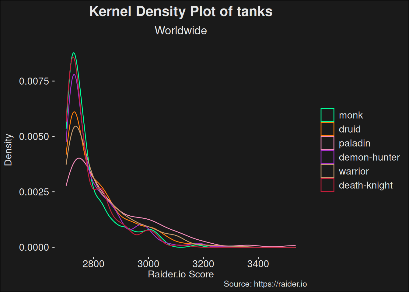
Code
players_topk |>filter(role =="tank") |>ggplot(aes(x = score, color = class)) +geom_density() +scale_color_manual(values = wow_colors) +scale_y_continuous("Density") +labs(title ="Kernel Density Plot of tanks",subtitle ="Worldwide",x ="Raider.io Score",caption ="Source: https://raider.io" )
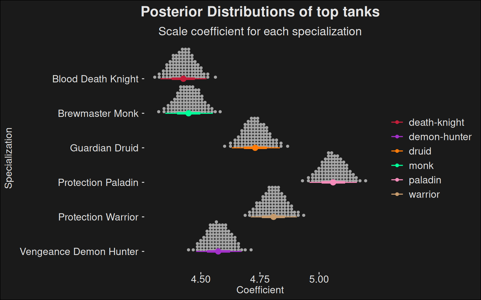
Code
fit |>recover_types(data_top) |>spread_draws(b[class_spec]) |>inner_join(spec_names, by =c("class_spec"="key")) |>filter(role =="tank") |>ggplot(aes(y =fct_rev(class_spec.str), x = b, color = key.class)) +stat_dotsinterval(quantiles =100) +scale_color_manual(values = wow_colors) +scale_fill_manual(values = wow_colors) +labs(title ="Posterior Distributions of top tanks",subtitle ="Scale coefficient for each specialization",x ="Coefficient",y ="Specialization" )
Warning: No shared levels found between `names(values)` of the manual scale and the
data's fill values.
8.4.3 DPS
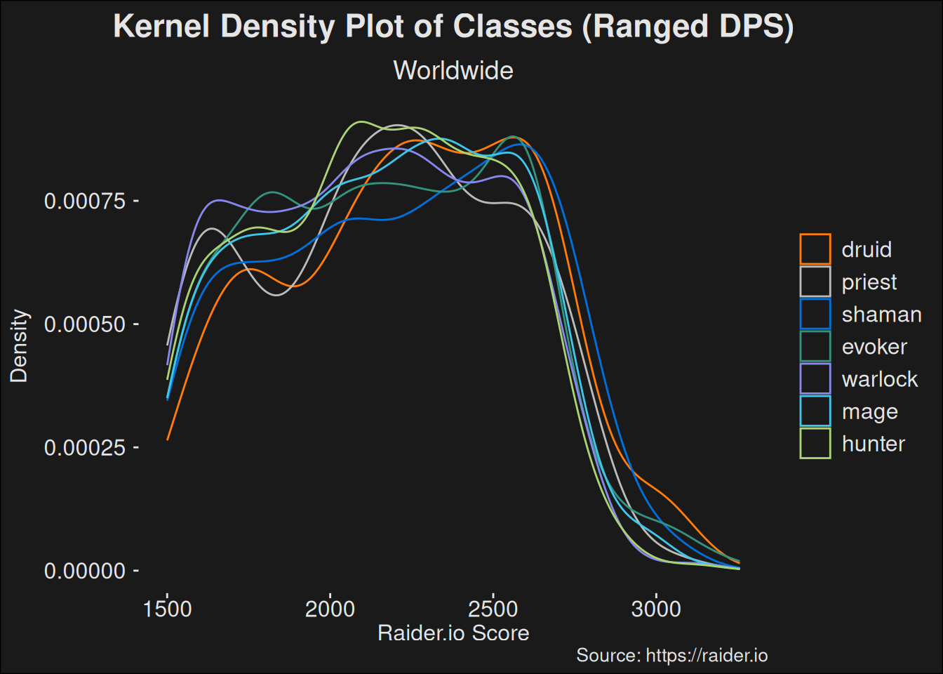
Likewise, for DPS, we only show the results.
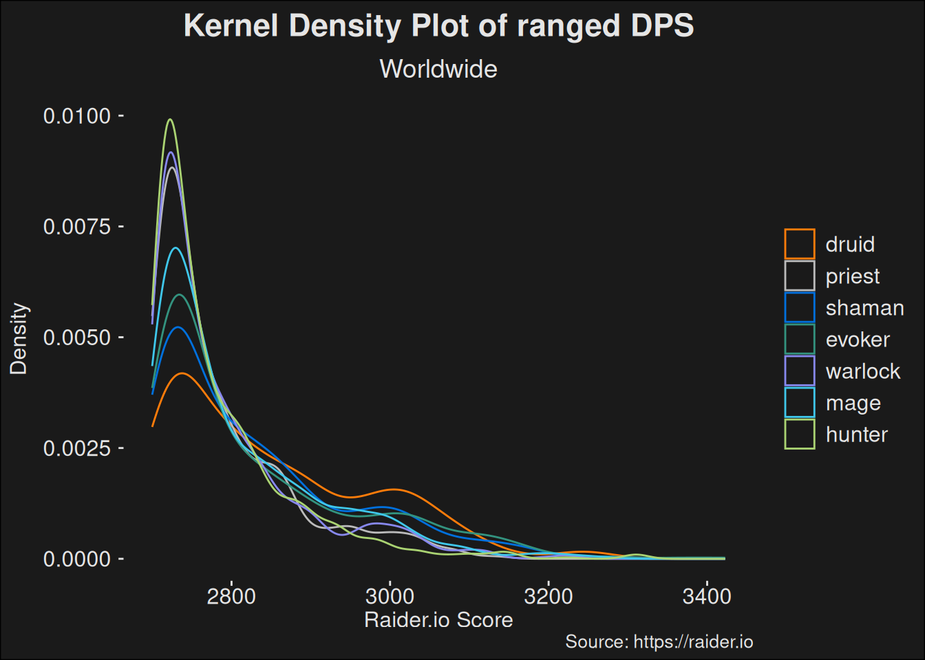
Code
players_topk |>filter(role =="dps"& is_ranged =="Yes") |>ggplot(aes(x = score, color = class)) +geom_density() +scale_color_manual(values = wow_colors) +scale_y_continuous("Density") +labs(title ="Kernel Density Plot of ranged DPS",subtitle ="Worldwide",x ="Raider.io Score",caption ="Source: https://raider.io" )
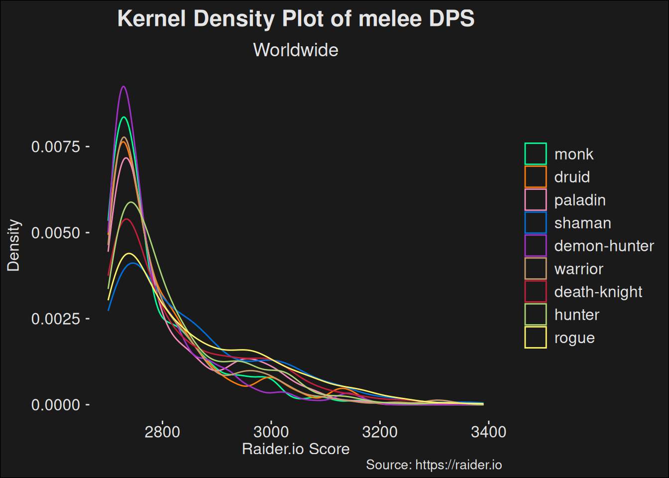
Code
players_topk |>filter(role =="dps"& is_ranged =="No") |>ggplot(aes(x = score, color = class)) +geom_density() +scale_color_manual(values = wow_colors) +scale_y_continuous("Density") +labs(title ="Kernel Density Plot of melee DPS",subtitle ="Worldwide",x ="Raider.io Score",caption ="Source: https://raider.io" )
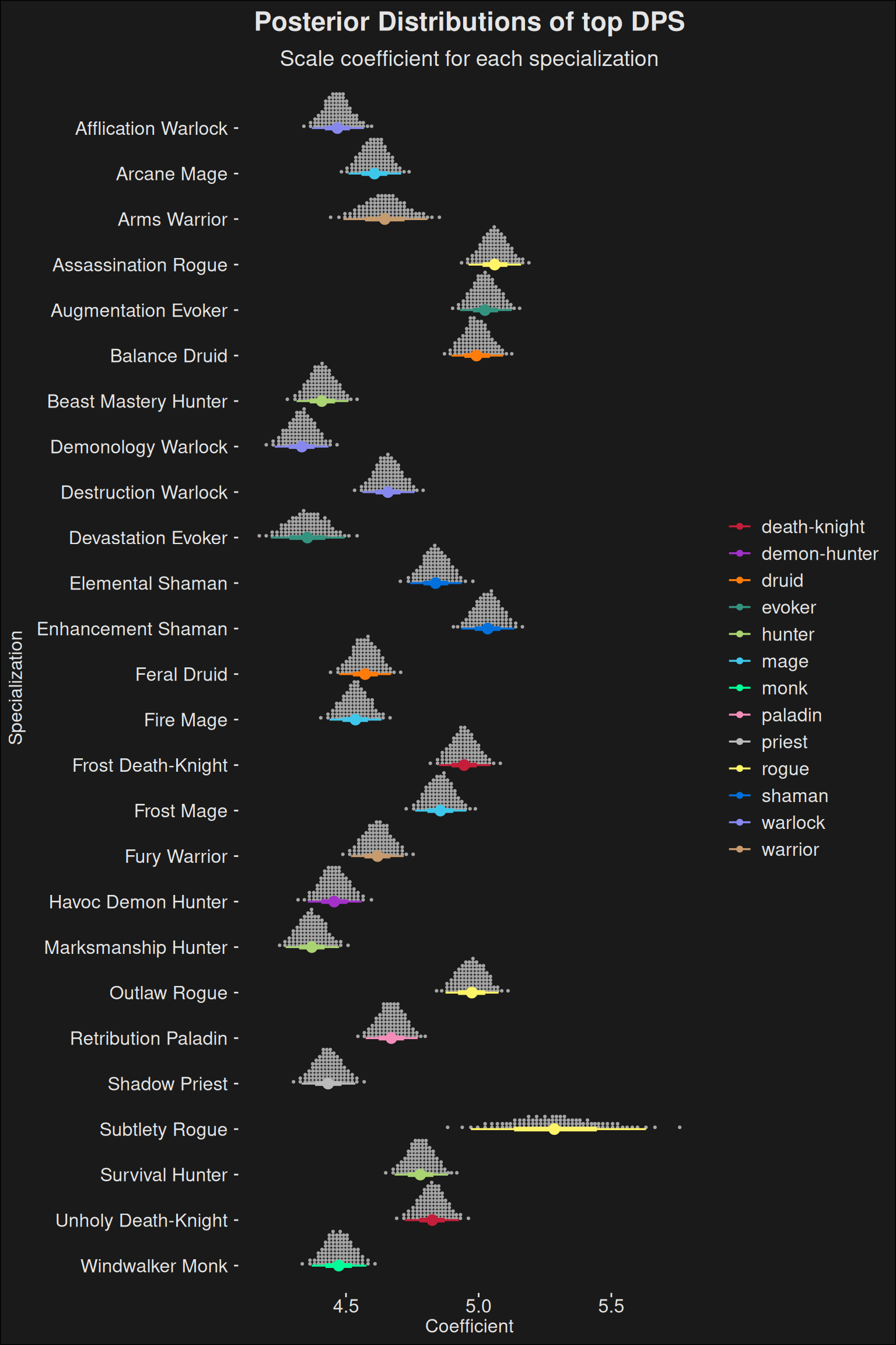
Code
fit |>recover_types(data_top) |>spread_draws(b[class_spec]) |>inner_join(spec_names, by =c("class_spec"="key")) |>filter(role =="dps") |>ggplot(aes(y =fct_rev(class_spec.str), x = b, color = key.class)) +stat_dotsinterval(quantiles =100) +scale_color_manual(values = wow_colors) +scale_fill_manual(values = wow_colors) +labs(title ="Posterior Distributions of top DPS",subtitle ="Scale coefficient for each specialization",x ="Coefficient",y ="Specialization" )
Warning: No shared levels found between `names(values)` of the manual scale and the
data's fill values.
8.4.4 Summary
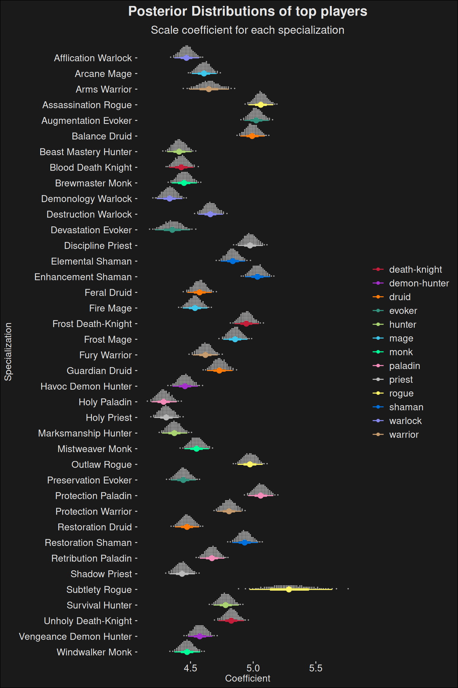
Finally, we have one big plot with every specialization. It allows you to answer questions across player roles. For instance if the best tank spec scores higher than the best healer spec.
Code
fit |>recover_types(data_top) |>spread_draws(b[class_spec]) |>inner_join(spec_names, by =c("class_spec"="key")) |>ggplot(aes(y =fct_rev(class_spec.str), x = b, color = key.class)) +stat_dotsinterval(quantiles =100) +scale_color_manual(values = wow_colors) +scale_fill_manual(values = wow_colors) +labs(title ="Posterior Distributions of top players",subtitle ="Scale coefficient for each specialization",x ="Coefficient",y ="Specialization" )
Warning: No shared levels found between `names(values)` of the manual scale and the
data's fill values.
8.4.5 Role split
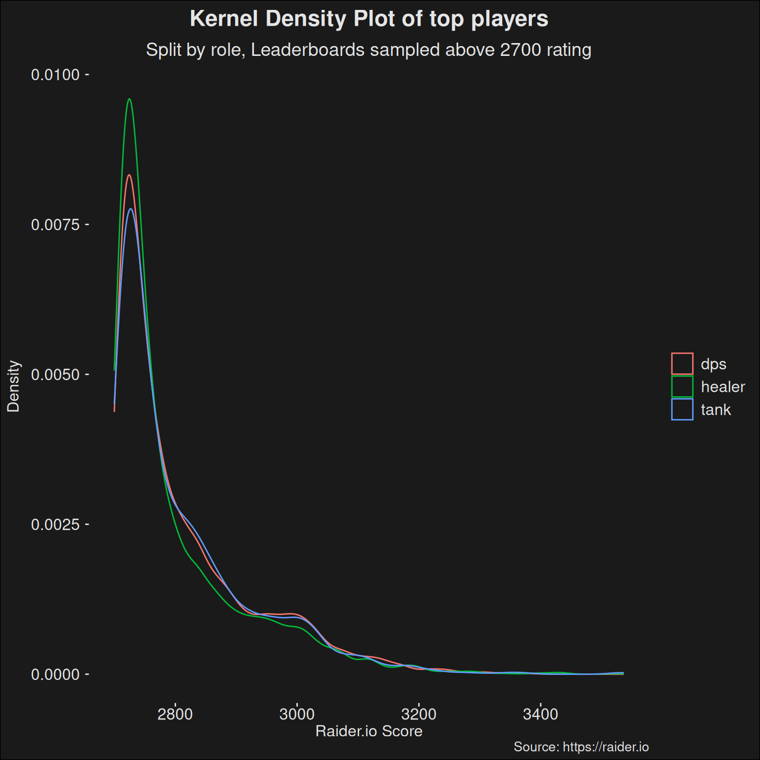
We can split the top players into roles as well and look at where that takes us. There may be differences compared to the more general population.
Code
players_topk |>ggplot(aes(x = score, color = role)) +geom_density() +scale_y_continuous("Density") +labs(title ="Kernel Density Plot of top players",subtitle ="Split by role, Leaderboards sampled above 2700 rating",x ="Raider.io Score",caption ="Source: https://raider.io" )
fit <- cmdstanr::as_cmdstan_fit(res_role$output_files())
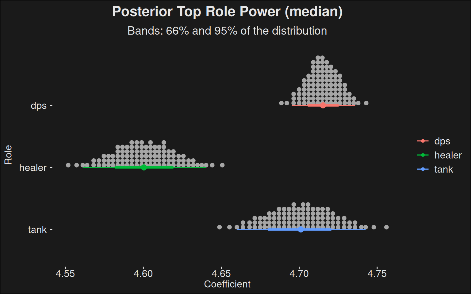
Code
fit |>recover_types(data) |>spread_draws(b[role]) |>ggplot(aes(y =fct_rev(role), x = b, color = role)) +stat_dotsinterval(quantiles =100) +labs(title ="Posterior Top Role Power (median)",subtitle ="Bands: 66% and 95% of the distribution",y ="Role",x ="Coefficient" )